Pressure-Temperature Profiles
In this notebook, we summarise the main pressure-temperature (P-T) profiles in POSEIDON.
Madhu
From Madhusudhan & Seager (2009), Equations 1 and 2 (https://ui.adsabs.harvard.edu/abs/2009ApJ…707…24M/abstract)
Guillot
From Guillot (2010), Equation 29 (https://ui.adsabs.harvard.edu/abs/2010A%26A…520A..27G/abstract)
Two versions: Guillot (redistribution factor f = 0.25 for terminators or directly imaged exoplanets) and Dayside Guillot (f = 0.5 for hot Jupiter daysides)
Line
From Line et al (2013), Equation 13 (https://ui.adsabs.harvard.edu/abs/2013ApJ…775..137L/abstract)
Pelletier
From Pelletier et al (2021), (Section 3.5) (https://ui.adsabs.harvard.edu/abs/2021AJ….162…73P/abstract)
Uses ‘knots’ to fit the PT profile with a second derivative penalty. Used for retrievals.
Slope
From Piette & Madhusudhan (2021) (https://ui.adsabs.harvard.edu/abs/2020MNRAS.497.5136P/abstract)
Other, more simple, profiles (such as an isotherm or gradient profile are also covered in previous tutorials).
If you use any of the following profiles, please cite the pertinent work above.
Configure Forward Model
We use HD 189733b to showcase how to define the new PT profiles
[1]:
from POSEIDON.constants import R_Sun, R_J, M_J
from POSEIDON.core import create_star, create_planet, define_model, wl_grid_constant_R
import numpy as np

#***** Model wavelength grid *****#

wl_min = 0.2    # Minimum wavelength (um)
wl_max = 30     # Maximum wavelength (um)
R = 5000        # Spectral resolution of grid

# We need to provide a model wavelength grid to initialise instrument properties
wl_1 = np.linspace(wl_min, 1.0, 1000)[:-1]
wl_2 = wl_grid_constant_R(1.0, wl_max, R)
wl_2 = wl_2[1:]    # Indexing to avoid 1.0 um being repeated twice
wl = np.concatenate((wl_1, wl_2))

#***** Define planet properties *****#

planet_name = 'HD 189733b'  # Planet name used for plots, output files etc.

R_p = 1.13*R_J    # Planetary radius (m)
M_p = 1.129*M_J   # Planetary mass (kg)
T_eq = 1200       # Equilibrium temperature (K)

planet = create_planet(planet_name, R_p, mass = M_p, T_eq = T_eq)

#***** Define stellar properties *****#

R_s = 0.78*R_Sun   # Stellar radius (m)
T_s = 5014         # Stellar effective temperature (K)
Met_s = 0.13       # Stellar metallicity [log10(Fe/H_star / Fe/H_solar)] <--- note: for PHOENIX, only the solar metallicity models are used
log_g_s = 4.58     # Stellar log surface gravity (log10(cm/s^2) by convention)

# Create the stellar object
star = create_star(R_s, T_s, log_g_s, Met_s, wl = wl, stellar_grid = 'phoenix')
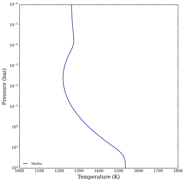
Madhusudhan & Seager
This profile has six free parameters: \(a_1\), \(a_2\), \(\log P_1\), \(\log P_2\), \(\log P_3\), and \(T_{\rm{ref}}\).
With the six parameters, a three region pressure-temperature profile is formulated.
\(P = P_0 e^{a_1 \sqrt{T-T_0}} \qquad (P_0 < P < P_1) \qquad (\mathrm{Region~1})\)
\(P = P_2 e^{a_2 \sqrt{T-T_2}} \qquad (P_1 < P < P_3) \qquad (\mathrm{Region~2})\)
\(T = T_3 \qquad (P < P_3) \qquad (\mathrm{Region~3})\)
where \(P_0\) and \(T_0\) are the pressure and temperature at the top of the atmosphere, \(P_{1,3}\) and \(T_{1,3}\) are specified at region boundaries, and \(P_2\) and \(T_2\) encode a potential temperature inversion point.
Temperature gradients are controlled by \(a_1\) and \(a_2\).
The regions are defined by \(P_1\), \(P_2\), \(P_3\) (\(P_0\) is given by the top of atmosphere pressure).
We note that POSEIDON allows the user to specify an arbitrary reference pressure at which the \(T_{\rm{ref}}\) parameter is defined, while the original Madhusudhan & Seager (2009) paper fixed this parameter to the top-of-atmosphere (\(T_0\)).
[2]:
# Madhusudhan & Seager

model_name_Madhu = 'Madhu'

bulk_species = ['H2', 'He']
param_species = []

# Create the model object
model_Madhu = define_model(model_name_Madhu, bulk_species, param_species,
                           PT_profile = 'Madhu')

print(model_Madhu['PT_param_names'])
['a1' 'a2' 'log_P1' 'log_P2' 'log_P3' 'T_ref']
[3]:
from POSEIDON.core import make_atmosphere

# Atmospheric pressure grid
P_min = 1.0e-6   # 1 ubar
P_max = 100      # 100 bar
N_layers = 100   # 100 layers

# Let's space the layers uniformly in log-pressure
P = np.logspace(np.log10(P_max), np.log10(P_min), N_layers)

# Specify the reference pressure
P_ref = 1   # The R_p_ref parameter will be the radius at 1 bar

# Free parameters
R_p_ref =   1.12 * R_J

a1      =   0.48
a2      =   0.21
log_P1  =   -4.04
log_P2  =   -2.40
log_P3  =   1.33
T_ref   =   1221.6

P_Madhu = 1.0e-2    # Pressure where T_ref is defined

PT_params = np.array([a1,a2,log_P1,log_P2,log_P3,T_ref])
log_X_params = np.array([])
cloud_params = np.array([])

atmosphere_Madhu = make_atmosphere(planet, model_Madhu, P, P_ref, R_p_ref,
                                   PT_params, log_X_params, cloud_params,
                                   P_param_set = P_Madhu,         # <---- This default to 1e-2 bar for T_ref if not set
                                   )
[4]:
from POSEIDON.visuals import plot_PT

# Produce plots of atmospheric properties
fig_PT = plot_PT(planet, model_Madhu, atmosphere_Madhu, log_P_max = 2.0)
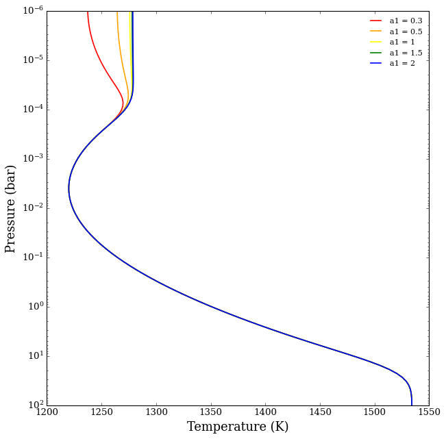
Lets vary one parameter at at a time.
\(a_1\) controls the temperature gradient from the top of the atmosphere to log_P1:
[5]:
from POSEIDON.visuals import vary_one_parameter_PT

param_name = 'a1'
vary_list = [0.3,0.5, 1, 1.5, 2]

vary_one_parameter_PT(model_Madhu, planet, param_name, vary_list,
                       P, P_ref, R_p_ref,
                       PT_params, log_X_params, cloud_params,
                       )
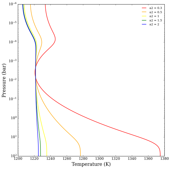
\(a_2\) controls the temperature gradient from log_P1 to log_P2:
[6]:
param_name = 'a2'
vary_list = [0.3,0.5, 1, 1.5, 2]

vary_one_parameter_PT(model_Madhu, planet, param_name, vary_list,
                       P, P_ref, R_p_ref,
                       PT_params, log_X_params, cloud_params,
                       )
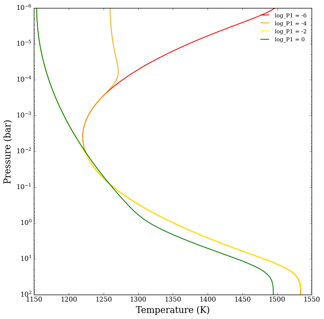
\(\log P_1\) is the pressure that defines the boundary between region 1 and 2:
[7]:
param_name = 'log_P1'
vary_list = [-6, -4, -2, 0]

vary_one_parameter_PT(model_Madhu, planet, param_name, vary_list,
                       P, P_ref, R_p_ref,
                       PT_params, log_X_params, cloud_params,
                       )
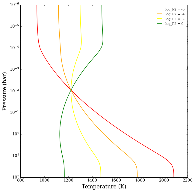
\(\log P_2\) is the pressure that defines a potential inversion point:
[8]:
param_name = 'log_P2'
vary_list = [-6, -4, -2, 0]

vary_one_parameter_PT(model_Madhu, planet, param_name, vary_list,
                       P, P_ref, R_p_ref,
                       PT_params, log_X_params, cloud_params,
                       )
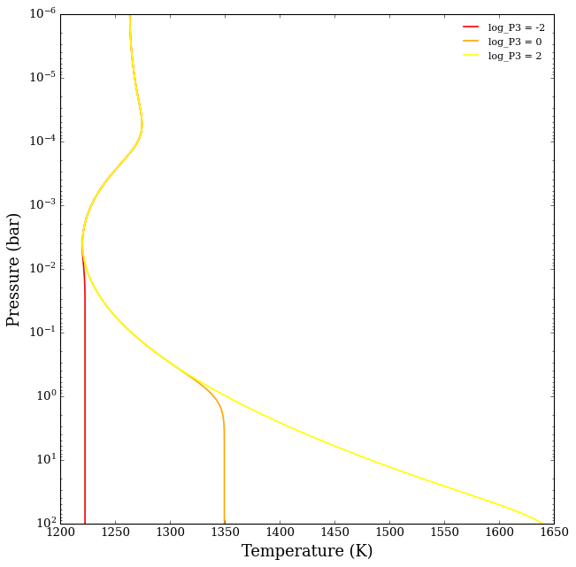
\(\log P_3\) is the pressure that defines the boundary between region 2 and 3:
[9]:
param_name = 'log_P3'
vary_list = [-2, 0, 2]

vary_one_parameter_PT(model_Madhu, planet, param_name, vary_list,
                       P, P_ref, R_p_ref,
                       PT_params, log_X_params, cloud_params,
                       )
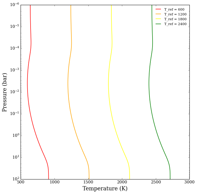
\(T_{\rm{ref}}\) is the temperature at a reference pressure (here 10 mbar):
[10]:
param_name = 'T_ref'
vary_list = [600, 1200, 1800, 2400]

vary_one_parameter_PT(model_Madhu, planet, param_name, vary_list,
                       P, P_ref, R_p_ref,
                       PT_params, log_X_params, cloud_params,
                       )
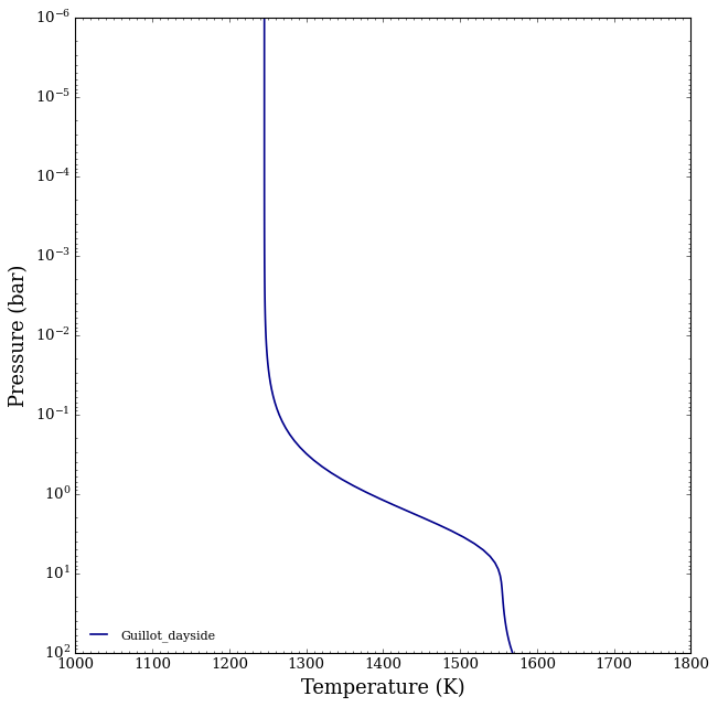
Dayside Guillot
This profile has four free parameters:
\(\log \kappa_{IR}\): The ‘infrared’ opacity
\(\log \gamma\): The ratio between optical and IR opacity
\(T_{\rm{int}}\): Internal temperature
\(T_{\rm{equ}}\): ‘Equilibrium’ temperature
where the free parameters are used to compute
\(T_{irr} = \sqrt{2}T_{eq}\), and the `infrared optical depth’, \(\tau = P \kappa_{IR}/g\)
which are plugged into
\(T^4 = \frac{3T_{int}^4}{4} \left(\frac{2}{3} + \tau\right) \notag \hspace{2pt} + f\frac{3T_{irr}^4}{4}\left(\frac{2}{3} + \frac{1}{\gamma\sqrt{3}} + \left(\frac{\gamma}{\sqrt{3}}-\frac{1}{\gamma\sqrt{3}}\right)e^{-\gamma\tau\sqrt{3}}\right)\)
[11]:
# Guillot Dayside

model_name_Guillot_dayside = 'Guillot_dayside'

bulk_species = ['H2', 'He']
param_species = []

# Create the model object
model_Guillot_dayside = define_model(model_name_Guillot_dayside, bulk_species, param_species,
                                     PT_profile = 'Guillot_dayside')

print(model_Guillot_dayside['PT_param_names'])
['log_kappa_IR' 'log_gamma' 'T_int' 'T_equ']
Lets set up some parameters and an atmosphere object
[12]:
from POSEIDON.core import make_atmosphere

# Atmospheric pressure grid
P_min = 1.0e-6   # 1 ubar
P_max = 100      # 100 bar
N_layers = 100   # 100 layers

# Let's space the layers uniformly in log-pressure
P = np.logspace(np.log10(P_max), np.log10(P_min), N_layers)

# Specify the reference pressure
P_ref = 1   # The R_p_ref parameter will be the radius at 1 bar

# Free parameters
R_p_ref = 1.12 * R_J

log_kappa_IR =   -4.83
log_gamma    =   -0.41
T_int        =   262.8
T_equ        =   1158.0

PT_params = np.array([log_kappa_IR, log_gamma, T_int, T_equ])
log_X_params = np.array([])
cloud_params = np.array([])

atmosphere_Guillot_dayside = make_atmosphere(planet, model_Guillot_dayside, P, P_ref, R_p_ref,
                                             PT_params, log_X_params, cloud_params)
[13]:
# Produce plots of atmospheric properties
fig_PT = plot_PT(planet, model_Guillot_dayside, atmosphere_Guillot_dayside, log_P_max = 2.0)
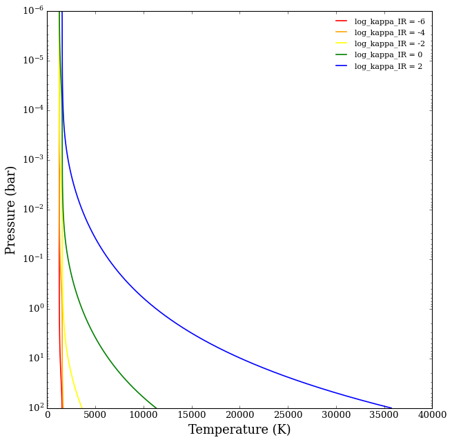
Lets see what varying the different parameters does.
[14]:
param_name = 'log_kappa_IR'
vary_list = [-6,-4,-2,0,2]

vary_one_parameter_PT(model_Guillot_dayside, planet, param_name, vary_list,
                       P, P_ref, R_p_ref,
                       PT_params, log_X_params, cloud_params,
                       )
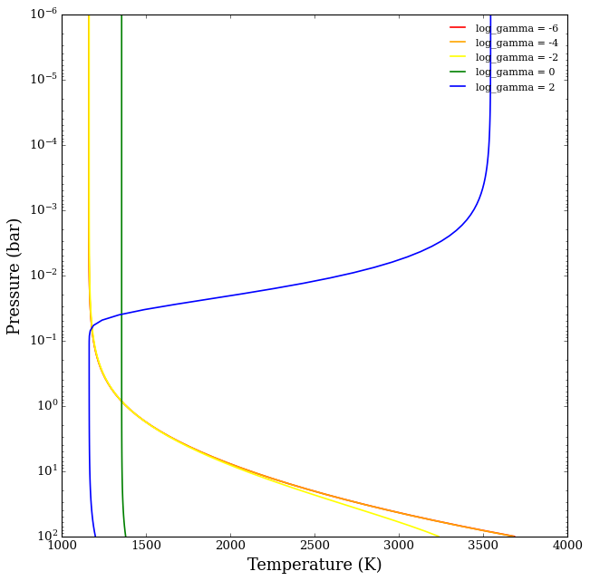
[15]:
param_name = 'log_gamma'
vary_list = [-6,-4,-2,0,2]

vary_one_parameter_PT(model_Guillot_dayside, planet, param_name, vary_list,
                       P, P_ref, R_p_ref,
                       PT_params, log_X_params, cloud_params,
                       )
[16]:
param_name = 'T_int'
vary_list = [0,200,400,600,1000]

vary_one_parameter_PT(model_Guillot_dayside, planet, param_name, vary_list,
                       P, P_ref, R_p_ref,
                       PT_params, log_X_params, cloud_params,
                       )
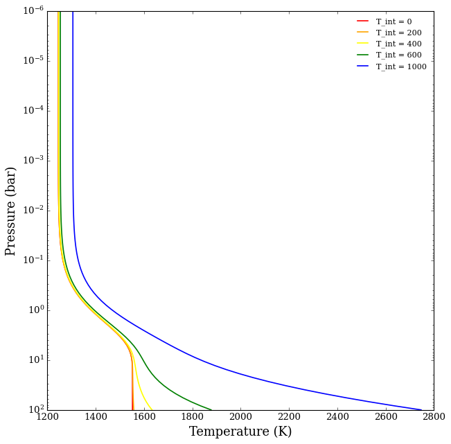
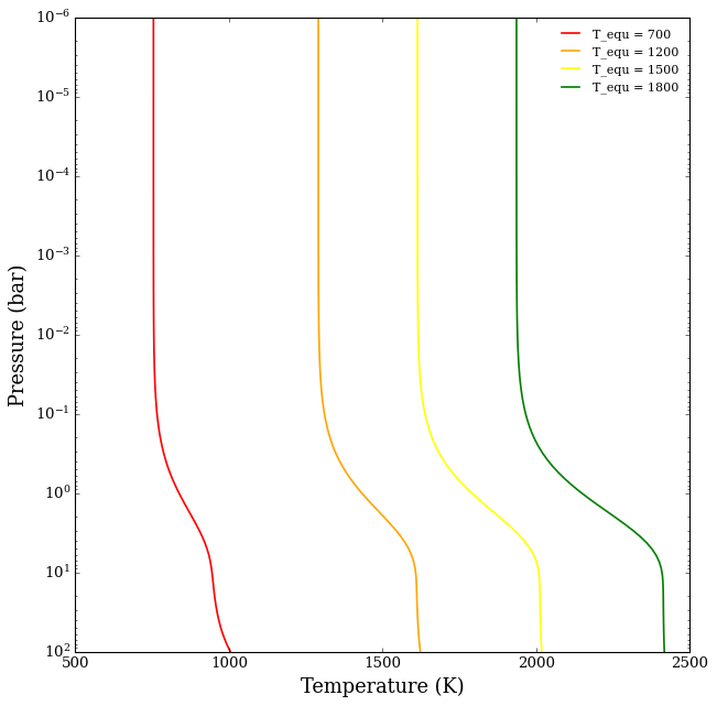
For normal profiles, \(T_{\rm{equ}}\) is typically the value for which the upper profile becomes isothermal.
[17]:
param_name = 'T_equ'
vary_list = [700,1200,1500,1800]

vary_one_parameter_PT(model_Guillot_dayside, planet, param_name, vary_list,
                       P, P_ref, R_p_ref,
                       PT_params, log_X_params, cloud_params,
                       )
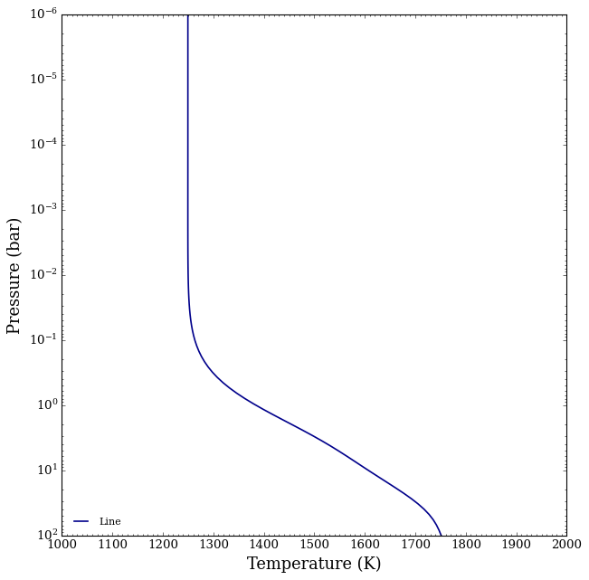
Line
This profile has six free parameters:
\(\log \kappa_{IR}\): The ‘infrared’ opacity
\(\log \gamma\): ratio between optical and IR opacity (channel 1)
\(\log \gamma_2\): ratio between optical and IR opacity (channel 2)
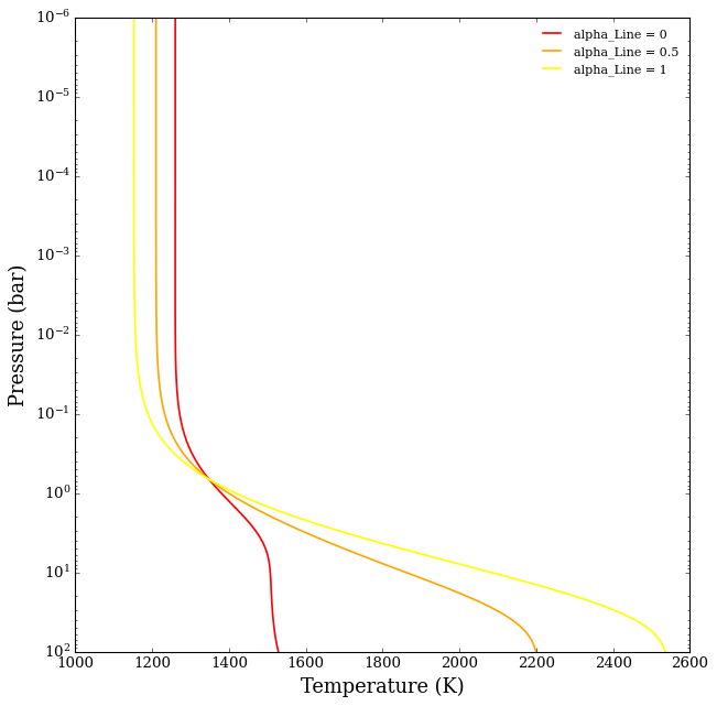
\(\alpha\): partitions the flux between channel 1 and 2 (ranges 0 to 1)
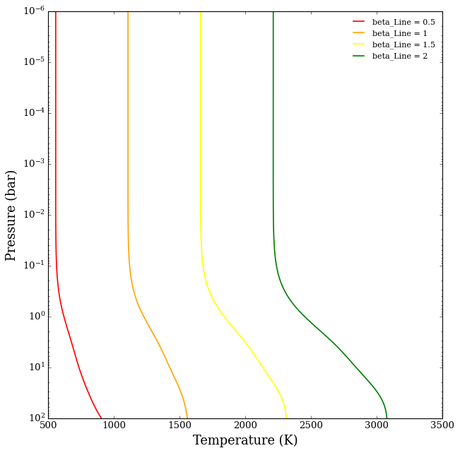
\(\beta\): a `catch-all’ term for heat redistribution, geometric arguments, emissivity, albedo, and errors in the equilibrium temperature
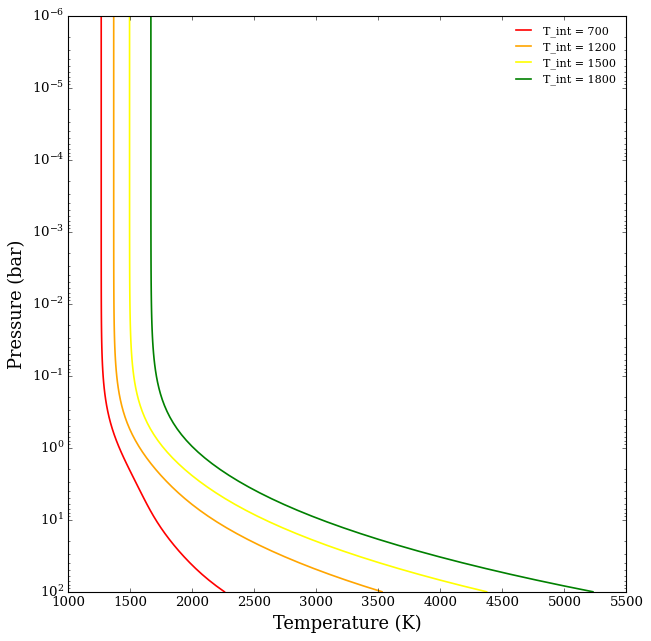
\(T_{\rm{int}}\): Internal temperature
where the free parameters are used to compute
\(T_{irr} = \beta T_{eq}\), and the `infrared optical depth’, \(\tau = P \kappa_{IR}/g\)
which are plugged into
$ T^4 = \frac{3T_{int}^4}{4}\left`(:nbsphinx-math:frac{2}{3}` + \tau\right) + \frac{3T_{irr}^4}{4}\left`(1-:nbsphinx-math:alpha`:nbsphinx-math:right):nbsphinx-math:xi{:nbsphinx-math:`gamma`}(:nbsphinx-math:`tau`) + :nbsphinx-math:`frac{3T_{irr}^4}{4}`:nbsphinx-math:`alpha`:nbsphinx-math:`xi`{\gamma`2}(:nbsphinx-math:tau`) $
where \(\xi\) is given by equation 14 in Line 2013.
Note that, unlike the Guillot profile, T_eq is NOT a free parameter and MUST be passed into the planet object. Additionally, the Line profile reduces down to the Guillot profile when alpha = 1.
[18]:
model_name_Line = 'Line'

#***** Define model *****#

bulk_species = ['H2', 'He']
param_species = []

# Create the model object
model_Line = define_model(model_name_Line, bulk_species, param_species,
                          PT_profile = 'Line')

print(model_Line['PT_param_names'])
['log_kappa_IR' 'log_gamma' 'log_gamma_2' 'alpha_Line' 'beta_Line' 'T_int']
[19]:
# Atmospheric pressure grid
P_min = 1.0e-6   # 1 ubar
P_max = 100      # 100 bar
N_layers = 100   # 100 layers

# Let's space the layers uniformly in log-pressure
P = np.logspace(np.log10(P_max), np.log10(P_min), N_layers)

# Specify the reference pressure
P_ref = 1   # The R_p_ref parameter will be the radius at 1 bar

# Free parameters
R_p_ref = 1.12 * R_J

log_kappa_IR =   -4.69
log_gamma    =   -0.31
log_gamma_2  =   -1.37
alpha_Line   =   0.11
beta_Line    =   1.13
T_int        =   258.8

PT_params = np.array([log_kappa_IR, log_gamma, log_gamma_2, alpha_Line, beta_Line, T_int])
log_X_params = np.array([])
cloud_params = np.array([])

atmosphere_Line = make_atmosphere(planet, model_Line, P, P_ref, R_p_ref,
                                  PT_params, log_X_params, cloud_params)
[20]:
# Produce plots of atmospheric properties
fig_PT = plot_PT(planet, model_Line, atmosphere_Line, log_P_max = 2.0)
[21]:
param_name = 'log_kappa_IR'
vary_list = [-6,-4,-2,0,2]

vary_one_parameter_PT(model_Line, planet, param_name, vary_list,
                       P, P_ref, R_p_ref,
                       PT_params, log_X_params, cloud_params,
                       )

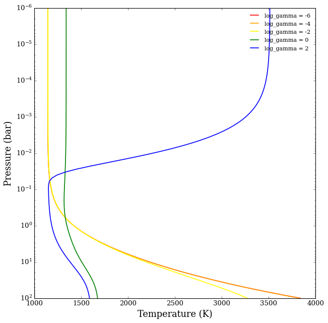
[22]:
param_name = 'log_gamma'
vary_list = [-6,-4,-2,0,2]

vary_one_parameter_PT(model_Line, planet, param_name, vary_list,
                       P, P_ref, R_p_ref,
                       PT_params, log_X_params, cloud_params,
                       )
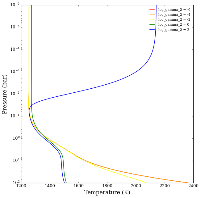
[23]:
param_name = 'log_gamma_2'
vary_list = [-6,-4,-2,0,2]

vary_one_parameter_PT(model_Line, planet, param_name, vary_list,
                       P, P_ref, R_p_ref,
                       PT_params, log_X_params, cloud_params,
                       )
[24]:
param_name = 'alpha_Line'
vary_list = [0,0.5,1]

vary_one_parameter_PT(model_Line, planet, param_name, vary_list,
                       P, P_ref, R_p_ref,
                       PT_params, log_X_params, cloud_params,
                       )
[25]:
param_name = 'beta_Line'
vary_list = [0.5,1,1.5,2]

vary_one_parameter_PT(model_Line, planet, param_name, vary_list,
                       P, P_ref, R_p_ref,
                       PT_params, log_X_params, cloud_params,
                       )
[26]:
param_name = 'T_int'
vary_list = [700,1200,1500,1800]

vary_one_parameter_PT(model_Line, planet, param_name, vary_list,
                       P, P_ref, R_p_ref,
                       PT_params, log_X_params, cloud_params,
                       )
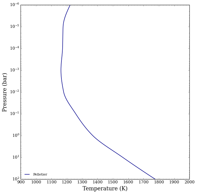
Pelletier
This profile has no set number of parameters.
It generated a uniform number of knots in between P_min and P_max.
Below, I have 9 knots, which will set the knots to be at each pressure level (2,1,0,-1,-2,-3,-4,-5,-6) bars.
T_1 represents the top of the atmosphere (1e-6 bars) and T_9 represents the bottom (1e2 bars)
Additionally, this model is primarily used in retrievals where it has a second derivative penalty on the PT profile (to prevent it from getting too wriggly)
This parameter is called sigma_s and is fit for during a retrieval. We reccomend setting a pretty tight prior on this parameter.
(For example, for 150 is a strict second derivative prior while 550 is not. The priors I set were +/- 20 that value.)
[27]:
model_name_Pelletier = 'Pelletier'

bulk_species = ['H2', 'He']
param_species = []

# Create the model object
model_Pelletier = define_model(model_name_Pelletier, bulk_species, param_species,
                               PT_profile = 'Pelletier',
                               number_P_knots = 9, PT_penalty = True)

print(model_Pelletier['PT_param_names'])
['T_1' 'T_2' 'T_3' 'T_4' 'T_5' 'T_6' 'T_7' 'T_8' 'T_9' 'sigma_s']
Results from sigma_s = 150
[28]:
# Atmospheric pressure grid
P_min = 1.0e-6   # 1 ubar
P_max = 100      # 100 bar
N_layers = 100   # 100 layers

# Let's space the layers uniformly in log-pressure
P = np.logspace(np.log10(P_max), np.log10(P_min), N_layers)

# Specify the reference pressure
P_ref = 1   # The R_p_ref parameter will be the radius at 1 bar

# Free parameters
R_p_ref =  1.12 * R_J

T_1     =   1222.7
T_2     =   1176.1
T_3     =   1172.5
T_4     =   1162.1
T_5     =   1179.5
T_6     =   1258.0
T_7     =   1368.8
T_8     =   1564.1
T_9     =   1775.1
sigma_s =   155.54

PT_params = np.array([T_1,T_2,T_3,T_4,T_5,T_6,T_7,T_8,T_9,sigma_s])
log_X_params = np.array([])
cloud_params = np.array([])

atmosphere_Pelletier = make_atmosphere(planet, model_Pelletier, P, P_ref, R_p_ref,
                                       PT_params, log_X_params, cloud_params)
[29]:
# Produce plots of atmospheric properties
fig_PT = plot_PT(planet, model_Pelletier, atmosphere_Pelletier, log_P_max = 2.0)
Now from the more ‘relaxed’ sigma_s = 550
[30]:
# Atmospheric pressure grid
P_min = 1.0e-6   # 1 ubar
P_max = 100      # 100 bar
N_layers = 100   # 100 layers

# Let's space the layers uniformly in log-pressure
P = np.logspace(np.log10(P_max), np.log10(P_min), N_layers)

# Specify the reference pressure
P_ref = 1   # The R_p_ref parameter will be the radius at 1 bar

# Free parameters
R_p_ref = 1.12 * R_J

T_1     =   835.0
T_2     =   732.9
T_3     =   982.5
T_4     =   1631.1
T_5     =   540.1
T_6     =   1378.0
T_7     =   2213.9
T_8     =   1957.9
T_9     =   1624.7
sigma_s =   552.50

PT_params = np.array([T_1,T_2,T_3,T_4,T_5,T_6,T_7,T_8,T_9,sigma_s])
log_X_params = np.array([])
cloud_params = np.array([])

atmosphere_Pelletier = make_atmosphere(planet, model_Pelletier, P, P_ref, R_p_ref,
                                       PT_params, log_X_params, cloud_params)
[31]:
# Produce plots of atmospheric properties
fig_PT = plot_PT(planet, model_Pelletier, atmosphere_Pelletier, log_P_max = 2.0)
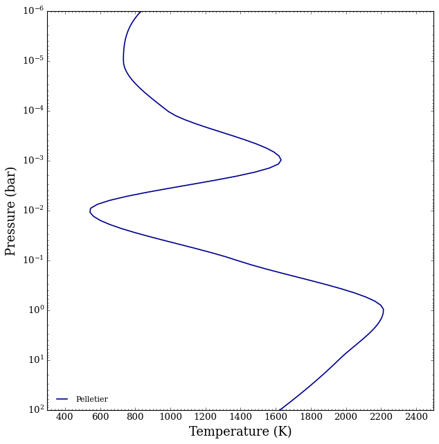
Its a lot more wriggly! Like we would expect.
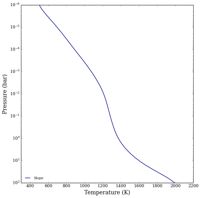
Slope
This profile has as many free parameters as the user specifies.
The original P-T profile, as defined in Piette & Madhusudhan (2021), fits for a photospheric temperature at 3.16 bars and a fixed number of \(\Delta\) T parameters between specific pressure anchor points (e.g., \(\Delta T\) from 10 to 1,mbar).
The implementation here allows the user to define the pressure of the photosphere and the pressure edges where the \(\Delta T\) parameters are defined (i.e., the number of \(\Delta T\) parameters is a user choice). This parameterization is much better suited than other P-T profiles at fitting a deep temperature adiabat with a decreasing temperature with height.
The slope profile explicitly assumes monotonically decreasing temperature with altitude and thus does not allow for thermal inversions (i.e., the \(\Delta T > 0\)).
Below: The photosphere is defined at 1e-1 bars with \(\Delta T_1\) from 1e-6 to 1e-5 bars, \(\Delta T_2\) from 1e-5 to 1e-4 bars, and so forth. \(T_{\rm{phot}}\) acts as the anchor point.
[32]:
model_name_slope = 'Slope'

#***** Define model *****#

bulk_species = ['H2', 'He']
param_species = []

# Create the model object
model_slope = define_model(model_name_slope, bulk_species, param_species,
                           PT_profile = 'slope',
                           log_P_slope_phot = -1,
                           log_P_slope_arr = [-6.0, -5.0, -4.0, -3.0, -2.0, 0.0, 1.0, 2.0,])
[33]:
from POSEIDON.core import make_atmosphere

# Atmospheric pressure grid
P_min = 1.0e-6   # 1 ubar
P_max = 100      # 100 bar
N_layers = 100   # 100 layers

# Let's space the layers uniformly in log-pressure
P = np.logspace(np.log10(P_max), np.log10(P_min), N_layers)

# Specify the reference pressure
P_ref = 1   # The R_p_ref parameter will be the radius at 1 bar

# Free parameters
R_p_ref = 1.12 * R_J

T_phot_PT =   1281.8
Delta_T_1 =   228.4
Delta_T_2 =   189.0
Delta_T_3 =   190.0
Delta_T_4 =   137.9
Delta_T_5 =   67.2
Delta_T_6 =   81.7
Delta_T_7 =   221.3
Delta_T_8 =   477.7

PT_params = np.array([T_phot_PT, Delta_T_1, Delta_T_2, Delta_T_3, Delta_T_4, Delta_T_5, Delta_T_6, Delta_T_7, Delta_T_8])
log_X_params = np.array([])
cloud_params = np.array([])

atmosphere_slope = make_atmosphere(planet, model_slope, P, P_ref, R_p_ref,
                                   PT_params, log_X_params, cloud_params)
[34]:
# Produce plots of atmospheric properties
fig_PT = plot_PT(planet, model_slope, atmosphere_slope, log_P_max = 2.0)