High-Resolution Spectroscopy
This tutorial demonstrates how to use POSEIDON’s forward model, TRIDENT, to generate grids of high spectral resolution models. We’ll assume familiarity with the main functions covered in “Generating Transmission Spectra”.
As a case study, here we consider WASP-76b — a hot Jupiter with many recent chemical species detections at high-resolution.
First, we define the main star and planet properties for the WASP-76 system (the values below are from exo.MAST).
[1]:
from POSEIDON.core import create_star, create_planet
from POSEIDON.constants import R_Sun, R_J
import numpy as np

#***** Define stellar properties *****#

R_s = 1.73*R_Sun      # Stellar radius (m)
T_s = 6250.0          # Stellar effective temperature (K)
Met_s = 0.23          # Stellar metallicity [log10(Fe/H_star / Fe/H_solar)]
log_g_s = 4.13        # Stellar log surface gravity (log10(cm/s^2) by convention)

# Create the stellar object
star = create_star(R_s, T_s, log_g_s, Met_s)

#***** Define planet properties *****#

planet_name = 'WASP-76b'  # Planet name used for plots, output files etc.

R_p = 1.82*R_J       # Planetary radius (m)
log_g_p = 2.8331     # Gravitational field of planet (cgs)
T_eq = 2182.12       # Equilibrium temperature (K)

# Create the planet object
planet = create_planet(planet_name, R_p, log_g = log_g_p, T_eq = T_eq)
Creating a High-Resolution Transmission Spectrum
Let’s first generate a high-resolution template model for \(\rm{Fe}\). We’ll assume a simple isothermal, cloud-free atmosphere with a solar \(\rm{Fe}\) abundance.
[2]:
from POSEIDON.core import define_model

#***** Define model *****#

model_name = 'Template_Fe'      # Model name used for plots, output files etc.

bulk_species = ['H2', 'He']     # H2 + He comprises the bulk atmosphere
param_species = ['Fe']          # We only need one chemical species for this template

# Create the model object
model = define_model(model_name, bulk_species, param_species,
                     PT_profile = 'isotherm', cloud_model = 'cloud-free')

# Check the free parameters defining this model
print("Free parameters: " + str(model['param_names']))
Free parameters: ['R_p_ref' 'T' 'log_Fe']
[3]:
from POSEIDON.core import make_atmosphere
import numpy as np

# Specify the pressure grid of the atmosphere
P_min = 1.0e-10   # Extend down to 0.1 nbar to avoid strong line cores 'clipping' at high-res
P_max = 100       # 100 bar
N_layers = 100    # 100 layers

# We'll space the layers uniformly in log-pressure
P = np.logspace(np.log10(P_max), np.log10(P_min), N_layers)

# Specify the reference pressure and radius
P_ref = 10.0   # Reference pressure (bar)
R_p_ref = R_p  # Radius at reference pressure

# Provide a specific set of model parameters for the atmosphere
PT_params = np.array([T_eq])        # Let's just use the equilibrium temperature
log_X_params = np.array([-4.5])     # -4.5 is roughly the solar Fe abundance (Asplund+2021)

# Generate the atmosphere
atmosphere = make_atmosphere(planet, model, P, P_ref, R_p_ref,
                             PT_params, log_X_params)
Line-by-line Transmission Spectra
We’ll now initialise POSEIDON’s opacity database at its native resolution (\(\Delta \tilde{\nu} = 0.01\) cm-1, equivalent to \(R = \lambda / \Delta \lambda = 10^6\) at 1 micron). Since this resolution is sufficient to resolve the line profiles of individual transition lines, such high spectral resolution models are commonly called ‘line-by-line’ models.
For our \(\rm{Fe}\) template, let’s generate a high-resolution model covering optical wavelengths.
[4]:
from POSEIDON.core import wl_grid_line_by_line
from POSEIDON.core import read_opacities

#***** Wavelength grid *****#

wl_min = 0.3      # Minimum wavelength (um)
wl_max = 1.0      # Maximum wavelength (um)

wl_high_res = wl_grid_line_by_line(wl_min, wl_max)

#***** Read opacity data *****#

opacity_treatment = 'line_by_line'

# Prepare high-resolution opacity data
opac_high_res = read_opacities(model, wl_high_res, opacity_treatment)
Notice how the opacity interpolation is almost instantaneous?
Unlike the opacity sampling mode (covered in “Generating Transmission Spectra with TRIDENT”), POSEIDON does not pre-interpolate cross sections in line-by-line mode (to conserve RAM). Instead, the cross sections are interpolated onto the specific layer pressure and temperatures of the atmosphere only when the user generates a spectrum. Hence, all of the computational burden occurs inside the compute_spectrum function.
The cell below should take around a minute to run.
[5]:
from POSEIDON.core import compute_spectrum

# Generate the high-resolution spectrum
spectrum_high_res = compute_spectrum(planet, star, model, atmosphere,
                                     opac_high_res, wl_high_res,
                                     spectrum_type = 'transmission',
                                     save_spectrum = True,             # Saves to ./POSEIDON_output/WASP-76b/spectra/
                                     disable_continuum = True)         # Turns off Rayleigh scattering and CIA
Reading in cross sections in line-by-line mode...
H2-H2 done
H2-He done
Fe done
Finished producing extinction coefficients
Note that we provided two new optional arguments to the compute_spectrum function:
save_spectrumoutputs a .txt file containing the model spectrum to the directory./POSEIDON_output/𝗽𝗹𝗮𝗻𝗲𝘁_𝗻𝗮𝗺𝗲/spectra/.disable_continuumturns off continuum opacity sources (i.e. Rayleigh scattering and CIA), which can be helpful for producing high-resolution absorption templates.
Finally, let’s plot our \(\rm{Fe}\) template.
[6]:
from POSEIDON.utility import plot_collection
from POSEIDON.visuals import plot_spectra

# Add both the high-res spectrum to a new plot collection
spectra = plot_collection(spectrum_high_res, wl_high_res, collection = [])

# Produce figure
fig = plot_spectra(spectra, planet, model, bin_spectra = False,  # Skip plotting a low resolution binned model
                   y_min = 1.1e-2, y_max = 2.1e-2,
                   spectra_labels = ['Fe absorption'], plt_label = 'Full Template')
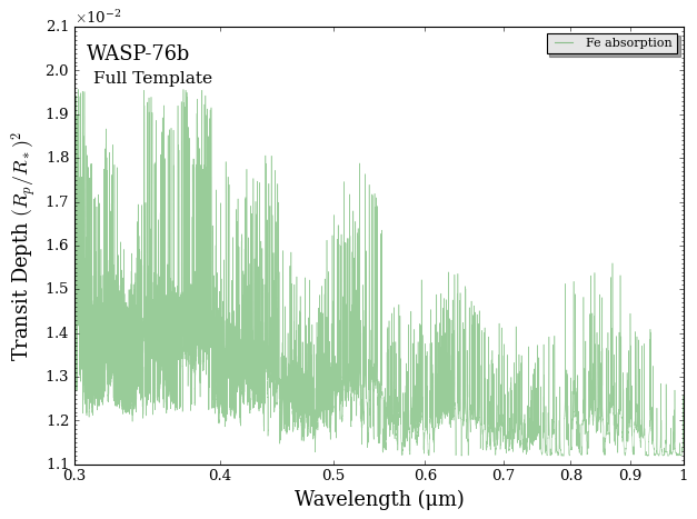
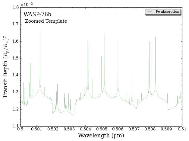
We can also zoom in on a narrow wavelength range to see individual \(\rm{Fe}\) lines.
[7]:
# Produce figure
fig = plot_spectra(spectra, planet, model, bin_spectra = False,
                   wl_min = 0.50, wl_max = 0.51,         # 0.50 to 0.51 um
                   y_min = 1.1e-2, y_max = 1.8e-2,
                   spectra_labels = ['Fe absorption'], plt_label = 'Zoomed Template')
Creating a Grid of High-Resolution Spectra
For cross correlation analyses, one will generally desire a grid of template models spanning different chemical species and atmospheric properties.
You can straightforwardly make a grid of high-resolution spectra by constructing a loop over atmospheric properties. The cell below provides an example to build a simple grid of model templates for \(\rm{Fe}\) and \(\rm{Ca}^{+}\) spanning 3 temperatures and 5 mixing ratios (for a total of 30 models).
Note:
Running the cell below will take around 30 minutes, with the grid using 2 GB of disk storage.
[8]:
from POSEIDON.core import define_model
from POSEIDON.core import make_atmosphere
from POSEIDON.core import wl_grid_line_by_line
from POSEIDON.core import read_opacities
from POSEIDON.core import compute_spectrum
import numpy as np

# Specify arrays of parameters to loop over
T_arr = np.array([2000, 2200, 2400])
log_X_arr = np.array([-8, -7, -6, -5, -4])
template_species = np.array(['Fe', 'Ca+'])

# Define model for grid
bulk_species = ['H2', 'He']      # H2 + He comprises the bulk atmosphere

# Specify the pressure grid of the atmosphere
P_min = 1.0e-10   # 0.1 nbar
P_max = 100       # 100 bar
N_layers = 100    # 100 layers

# We'll space the layers uniformly in log-pressure
P = np.logspace(np.log10(P_max), np.log10(P_min), N_layers)

# Specify the reference pressure and radius
P_ref = 10.0   # Reference pressure (bar)
R_p_ref = R_p  # Radius at reference pressure

#***** Wavelength grid *****#

wl_min = 0.3     # Minimum wavelength (um)
wl_max = 1.0     # Maximum wavelength (um)

wl_high_res = wl_grid_line_by_line(wl_min, wl_max)

#***** Read opacity data *****#

opacity_treatment = 'line_by_line'

model_count = 0   # Counter variable so user can track model grid progress

# Loop over chemical species, temperatures, and mixing ratios
for q in range(len(template_species)):
    for i in range(len(T_arr)):
        for j in range(len(log_X_arr)):

            model_count += 1

            # Load chemical species and atmospheric properties for this template
            param_species = [template_species[q]]
            T_i = T_arr[i]
            log_X_j = log_X_arr[j]

            # Define model name for this parameter combination
            model_name = param_species[0] + '_' + str(log_X_j) + '_T_' + str(T_i) + 'K'

            # Create the model object
            model = define_model(model_name, bulk_species, param_species,
                                 PT_profile = 'isotherm', cloud_model = 'cloud-free')

            # Prepare high-resolution opacity data
            opac_high_res = read_opacities(model, wl_high_res, opacity_treatment)

            # Store parameters in input array
            PT_params = np.array([T_i])
            log_X_params = np.array([[log_X_j]])

            # Generate the atmosphere
            atmosphere = make_atmosphere(planet, model, P, P_ref, R_p_ref,
                                         PT_params, log_X_params)

            # Compute the spectrum
            spectrum_high_res = compute_spectrum(planet, star, model, atmosphere,
                                                 opac_high_res, wl_high_res,
                                                 spectrum_type = 'transmission',
                                                 save_spectrum = True,
                                                 disable_continuum = True,
                                                 suppress_print = True)             # Suppress 'cross section done' print statements

            print("Model " + str(model_count) + "/" +
                  str(len(T_arr)*len(log_X_arr)*len(template_species)) + " done.")
Model 1/30 done.
Model 2/30 done.
Model 3/30 done.
Model 4/30 done.
Model 5/30 done.
Model 6/30 done.
Model 7/30 done.
Model 8/30 done.
Model 9/30 done.
Model 10/30 done.
Model 11/30 done.
Model 12/30 done.
Model 13/30 done.
Model 14/30 done.
Model 15/30 done.
Model 16/30 done.
Model 17/30 done.
Model 18/30 done.
Model 19/30 done.
Model 20/30 done.
Model 21/30 done.
Model 22/30 done.
Model 23/30 done.
Model 24/30 done.
Model 25/30 done.
Model 26/30 done.
Model 27/30 done.
Model 28/30 done.
Model 29/30 done.
Model 30/30 done.