Thermal Emission Retrievals of Bare Rocky Exoplanets
Tidally locked, hot, bare-rocky exoplanets provide a unique avenue to explore surface geology by probing mid-infrared absorption features characteristc of specific rocks.
In this tutorial, we explore how to perform retrieval analysis when assuming a bare rocky exoplanet with no atmosphere (though, we note that all the surface + atmosphere + clouds models featured in ‘Rocky Planets with Reflecting and Emitting Surfaces’ can be used in a retrieval, here we only explore planetary bodies without atmospheres in since, as we will see below, the retrieval run very fast compared to models with atmospheres and clouds).
This tutorial assumes a basic understanding of the ‘Atmospheric Retrievals with POSEIDON’ tutorial.
Note:
As of POSEIDON v1.4, there is a surface albedo database that is now included in the inputs folder. If you already have downloaded the v1.3 version of the inputs, and don’t want to redownload them, you can access the surface_reflectivities folder here to add it manually.
Download the surface_reflectivities.zip folder, unzip it, and add it to your inputs folder.
As of 1.4 you should have four top-level folders in inputs: stellar_grids, opacity, chemistry_grids, and surface_reflectivities.
Case Study: TOI 1685b Retrieval
Lets define the stellar and planetary properties for our system: TOI 1685b.
[1]:
from POSEIDON.constants import R_Sun, R_J, M_J, R_E, M_E
from POSEIDON.core import create_star, create_planet, load_data, define_model, \
                          wl_grid_constant_R, set_priors, read_opacities
from POSEIDON.visuals import plot_data, plot_spectra_retrieved, plot_PT_retrieved
from POSEIDON.retrieval import run_retrieval
from POSEIDON.utility import read_retrieved_spectrum, read_retrieved_PT, \
                             read_retrieved_log_X, plot_collection
from POSEIDON.corner import generate_cornerplot

import numpy as np
from scipy.constants import au
from scipy.constants import parsec as pc

#***** Model wavelength grid *****#

wl_min = 0.3     # Minimum wavelength (um)
wl_max = 15     # Maximum wavelength (um)
R = 1000         # Spectral resolution of grid

wl = wl_grid_constant_R(wl_min, wl_max,R)

#***** Define planet properties *****#

planet_name = 'TOI-1685b'  # Planet name used for plots, output files etc.

R_p = 1.468*R_E    # Planetary radius (m)
M_p = 3.03*M_E
d = 37.6153*pc
a_p = 0.01138*au   # For reflection, we have to set the semi-major axis

# Create the planet object
planet = create_planet(planet_name, R_p, mass = M_p, a_p = a_p)


#***** Define stellar properties *****#

R_s = 0.4555*R_Sun      # Stellar radius (m)
T_s = 3575        # Stellar effective temperature (K)
Met_s = 0.3          # Stellar metallicity [log10(Fe/H_star / Fe/H_solar)] <--- note: for PHOENIX, only the solar metallicity models are used
log_g_s = 4.778       # Stellar log surface gravity (log10(cm/s^2) by convention)

# Create the stellar object
star = create_star(R_s, T_s, log_g_s, Met_s, wl = wl, stellar_grid = 'phoenix')
Loading JWST Simulated Data from Online Version of PANDEXO
Here, we have created a simulated JWST MIRI dataset with the online version of PANDEXO (https://exoctk.stsci.edu/pandexo/calculation/new)
The online version of PANDEXO is a great alternative to the downloadable version featured in `Supporting a JWST Proposal with POSEIDON’ tutorial.
In order to make the simulated data spectrum, we
Resolved the target from its name
Used the default stellar spectrum from phoenix
Uploaded a forward model spectrum made in POSEIDON (micron, Fp/Fs) [we will keep the forward model here a secret, as to not ruin the suprise of the retrieval analysis]
Baseline of 1, with 10 transits
MIRI LRS Spectroscopy, Slitless LRS, Optimize, 80% Full Well, and a Constant Minimum Noise of 0
This process is a bit different than the one done in the ‘Supporting a JWST Proposal with POSEIDON’ tutorial. In particular, we are scattering simualted data around a spectrum that we then bin down, instead of using simulated error bars to generate synthetic data around.
Lets load in our pandexo output!
[2]:
#***** Specify data location and instruments  *****#

data_dir = '../../../POSEIDON/reference_data/observations/TOI-1685b'         # Change this to where your data is stored
datasets = ['TOI-1685b-MIRI-PandexoOutput.txt']  # Found in reference_data/observations
instruments = ['JWST_MIRI_LRS']             # Instruments corresponding to the data

# Load dataset, pre-load instrument PSF and transmission function
data = load_data(data_dir, datasets, instruments, wl, skiprows = 1)

# Plot our data
fig_data = plot_data(data, planet_name, y_unit = 'eclipse_depth')
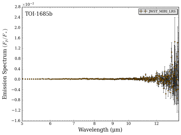
That looks very noisy. Lets go ahead and bin it down!
We have introduced a new function that takes pandexo’s output and bins it down.
Since we often want to try many different binning resolutions, we also specify a saved_directory to store the binned down data at.
Note that, for MIRI data, you have to specify that it is MIRI since pandexo returns a txt file that is flipped in wavelength compared to other datasets.
[ ]:
from POSEIDON.instrument import create_binned_down_data_from_pandexo

data_dir = '../../../POSEIDON/reference_data/observations/TOI-1685b'
saved_directory = data_dir + '/binned_spectra/' #<- specify where to save the data at
file_name = 'TOI-1685b-MIRI-PandexoOutput.txt'  #<- name of the file we are loading to bin down
R_to_bin = 15                                   #<- R to bin down to, here an R of 15

create_binned_down_data_from_pandexo(file_name,
                            wl, R_to_bin,
                            stored_directory=data_dir,
                            saved_directory = saved_directory,
                            is_miri = True,)
Lets see what this dataset looks like
[4]:
#***** Specify data location and instruments  *****#

data_dir = '../../../POSEIDON/reference_data/observations/TOI-1685b/binned_spectra'         # Change this to where your data is stored
datasets = ['TOI-1685b-MIRI-PandexoOutput_R15.txt']  # Found in reference_data/observations
instruments = ['JWST_MIRI_LRS']             # Instruments corresponding to the data

# Load dataset, pre-load instrument PSF and transmission function
data = load_data(data_dir, datasets, instruments, wl, skiprows = 1)

# Plot our data
fig_data = plot_data(data, planet_name, y_unit = 'eclipse_depth')
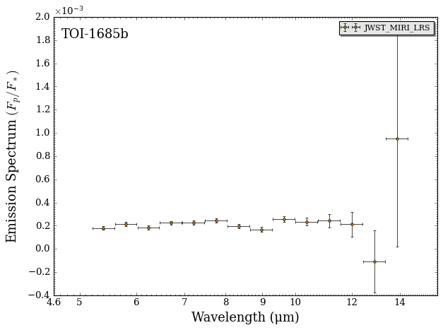
Since MIRI’s sensitivity falls off extremely at the longest wavlenegths, lets zoom-in a bit
[5]:
#***** Specify data location and instruments  *****#

data_dir = '../../../POSEIDON/reference_data/observations/TOI-1685b/binned_spectra'         # Change this to where your data is stored
datasets = ['TOI-1685b-MIRI-PandexoOutput_R15.txt']  # Found in reference_data/observations
instruments = ['JWST_MIRI_LRS']             # Instruments corresponding to the data

# Load dataset, pre-load instrument PSF and transmission function
data = load_data(data_dir, datasets, instruments, wl, skiprows = 1)

# Plot our data
fig_data = plot_data(data, planet_name, y_unit = 'eclipse_depth', y_min = 0, y_max = 3e-4)
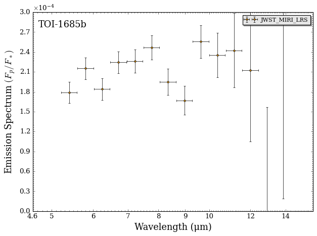
Great! We now have binned down synthetic data to run a retrieval on.
Surface Composition and Geological Implications
Now, lets set up our forward model for the retrieval. For bare rocks we are interested in two main properties: surface temperature, and surface composition.
For surface retrievals, lets try three different surface albedos simultaenously and see which the dataset favors the most.
To do this, we define three surface components:
Black = Albedo of 0 at all wavelengths. Would be synonymous with a non-detection of surface geology, but helps in constraining a surface temperature.
Granite = A felsic (silica-rich) rock. In the Solar System, only Earth has a large amount of granite when compared to other rocky planets due to plate tectonics (where mafic crust is reprocessed as granitic continental crust). However, granite by itelf doesn’t always mean plate tectonics, as it could form due to a planet just being silica-rich from formation.
Basalt = A mafic rock. In the Solar System, basalts represent the most ubiqituous surface, as it is the natural consequence of what forms from the partial melting of ultramafic mantle material. If this pattern extends beyond the Solar System, we would expect basalts to be common as an exoplanet surface.
If you are more interested in how to start interpreting specific rocks in the context of exogeology, please check out Mullens et al (2026) Appendix material, which is also present in the surface albedo database!
CLR vs Uniform Priors for Surface Components
Surface component percentages can be defined in both linear (0-1) and log space. For the retrievals in this tutorial, we’ll demonstrate both for the uniform prior.
Uniform priors are the normal, default prior, where percentages for each surface component are drawn seperately and then normalized to 1.
The CLR (Center-Log Ratio) Prior can also be utilized for surfaces. This prior is useful when you can’t make any assumptions about which surface component will be the dominate surface component. In particular, this prior draws for N-1 surface component percentages, and fills the rest of the surface with the remaining surface component until they add up to 100%. In particular, it has less one less free parameter when compared to the uniform prior. Additionally, the CLR prior requires the percentages to be in log-space.
In this tutorial, we will demonstrate both the uniform and the CLR prior.
As described in Mullens et al. (2026), both uniform and CLR priors have advantages and disadvantages. The CLR prior (with log percentages) is useful in determining which surface is most likely the bulk surface component, while the uniform prior (with linear percentages) is useful in discovering degeneracies that come from linearly combining different albedo datasets.
Model Definitions
[ ]:
model_name_linear_uniform = 'TOI-1685b-Linear-Percentages'

#***** Define model *****#

bulk_species = []
param_species = []

# List the surface components here
surface_components = ['Black','Granitoid_H12','Tholeiitic_basalt_H25']

# Create the model object
model_linear_uniform = define_model(model_name_linear_uniform, bulk_species, param_species,
                            radius_unit = 'R_E', surface = True,  # <----- Set surface = True
                            reflection = True, thermal = True, thermal_scattering = True, # <----- Set reflection and thermal to True
                            surface_model = 'lab_data',           # <----- Set surface_model to 'lab_data'
                            surface_components = surface_components,  # <----- Input surface_components
                            disable_atmosphere = True,                # <----- Set disable_atmosphere = True for bare rocks
                            surface_percentage_option = 'linear',     # <----- Use linear percentages (0 to 1)
                            surface_percentage_apply_to = 'models')    # <----- Apply percentages to models (3 models for each spectra)

print(model_linear_uniform['param_names'])
['R_p_ref' 'T_surf' 'Black_percentage' 'Granitoid_H12_percentage'
 'Tholeiitic_basalt_H25_percentage']
[ ]:
model_name_log_uniform = 'TOI-1685b-Log-Percentages-Uniform'

#***** Define model *****#

bulk_species = []
param_species = []

# List the surface components here
surface_components = ['Black','Granitoid_H12','Tholeiitic_basalt_H25']

# Create the model object
model_log_uniform   = define_model(model_name_log_uniform, bulk_species, param_species,
                            radius_unit = 'R_E', surface = True,  # <----- Set surface = True
                            reflection = True, thermal = True, thermal_scattering = True, # <----- Set reflection and thermal to True
                            surface_model = 'lab_data',           # <----- Set surface_model to 'lab_data'
                            surface_components = surface_components,  # <----- Input surface_components
                            disable_atmosphere = True,                # <----- Set disable_atmosphere = True for bare rocks
                            surface_percentage_option = 'log',        # <----- Use log percentages
                            surface_percentage_apply_to = 'models')    # <----- Apply percentages to models (3 models for each spectra)

print(model_log_uniform['param_names'])
['R_p_ref' 'T_surf' 'log_Black_percentage' 'log_Granitoid_H12_percentage'
 'log_Tholeiitic_basalt_H25_percentage']
[ ]:
# Here we duplicate the model for the CLR prior

model_name_log_clr = 'TOI-1685b-Log-Percentages-CLR'

#***** Define model *****#

bulk_species = []
param_species = []

# List the surface components here
surface_components = ['Black','Granitoid_H12','Tholeiitic_basalt_H25']

# Create the model object
model_log_clr   = define_model(model_name_log_clr, bulk_species, param_species,
                            radius_unit = 'R_E', surface = True,  # <----- Set surface = True
                            reflection = True, thermal = True, thermal_scattering = True, # <----- Set reflection and thermal to True
                            surface_model = 'lab_data',           # <----- Set surface_model to 'lab_data'
                            surface_components = surface_components,  # <----- Input surface_components
                            disable_atmosphere = True,                # <----- Set disable_atmosphere = True for bare rocks
                            surface_percentage_option = 'log',        # <----- Use log percentages
                            surface_percentage_apply_to = 'models')    # <----- Apply percentages to models (3 models for each spectra)

print(model_log_clr['param_names'])
['R_p_ref' 'T_surf' 'log_Black_percentage' 'log_Granitoid_H12_percentage'
 'log_Tholeiitic_basalt_H25_percentage']
1. Uniform Prior, Linear Percentages
[ ]:
# Initialise prior type dictionary
prior_types = {}

# Specify uniform priors for all free parameters
prior_types['R_p_ref'] = 'uniform'
prior_types['T_surf'] = 'uniform' #<- Surface temperature

prior_types['Black_percentage'] = 'uniform'
prior_types['Granitoid_H12_percentage'] = 'uniform'
prior_types['Tholeiitic_basalt_H25_percentage'] = 'uniform'

# Initialise prior range dictionary
prior_ranges = {}

# Specify prior ranges for each free parameter
prior_ranges['R_p_ref'] = [0.9*R_p, 1.1*R_p]

prior_ranges['T_surf'] = [100,2000]

# Percentages range from 0 to 1, or 0 to 100%
prior_ranges['Black_percentage'] = [0,1]
prior_ranges['Granitoid_H12_percentage'] = [0,1]
prior_ranges['Tholeiitic_basalt_H25_percentage'] = [0,1]

# Create prior object for retrieval
priors = set_priors(planet, star, model_linear_uniform, data, prior_types, prior_ranges)
Lets run the retrieval.
Surface retrievals are very fast, since they do not need to compute atmospheric radiative transfer.
[ ]:
#***** Specify fixed atmospheric settings for retrieval *****#

# For bare rocks, P and opac arrays are empty
P = []
P_ref = []
opac = []

run_retrieval(planet, star, model_linear_uniform, opac, data, priors, wl, P, P_ref, R = R,
                spectrum_type = 'emission', sampling_algorithm = 'MultiNest',
                N_live = 500, verbose = True, resume = False)
POSEIDON now running 'TOI-1685b-Linear-Percentages'
*****************************************************
MultiNest v3.10
Copyright Farhan Feroz & Mike Hobson
Release Jul 2015
no. of live points = 500
dimensionality = 5
*****************************************************
Starting MultiNest
generating live points
live points generated, starting sampling
Acceptance Rate: 0.990991
Replacements: 550
Total Samples: 555
Nested Sampling ln(Z): -500.042794
Acceptance Rate: 0.980392
Replacements: 600
Total Samples: 612
Nested Sampling ln(Z): -457.751338
Acceptance Rate: 0.943396
Replacements: 650
Total Samples: 689
Nested Sampling ln(Z): -380.846297
Acceptance Rate: 0.919842
Replacements: 700
Total Samples: 761
Nested Sampling ln(Z): -324.388131
Acceptance Rate: 0.892857
Replacements: 750
Total Samples: 840
Nested Sampling ln(Z): -245.684053
Acceptance Rate: 0.854701
Replacements: 800
Total Samples: 936
Nested Sampling ln(Z): -153.022941
Acceptance Rate: 0.828460
Replacements: 850
Total Samples: 1026
Nested Sampling ln(Z): -101.870007
Acceptance Rate: 0.816697
Replacements: 900
Total Samples: 1102
Nested Sampling ln(Z): -57.049488
Acceptance Rate: 0.808511
Replacements: 950
Total Samples: 1175
Nested Sampling ln(Z): -27.717481
Acceptance Rate: 0.796178
Replacements: 1000
Total Samples: 1256
Nested Sampling ln(Z): 2.384433
Acceptance Rate: 0.794852
Replacements: 1050
Total Samples: 1321
Nested Sampling ln(Z): 23.114734
Acceptance Rate: 0.785153
Replacements: 1100
Total Samples: 1401
Nested Sampling ln(Z): 41.189163
Acceptance Rate: 0.775455
Replacements: 1150
Total Samples: 1483
Nested Sampling ln(Z): 58.467278
Acceptance Rate: 0.764331
Replacements: 1200
Total Samples: 1570
Nested Sampling ln(Z): 68.420132
Acceptance Rate: 0.758495
Replacements: 1250
Total Samples: 1648
Nested Sampling ln(Z): 77.635345
Acceptance Rate: 0.752750
Replacements: 1300
Total Samples: 1727
Nested Sampling ln(Z): 85.510435
Acceptance Rate: 0.745445
Replacements: 1350
Total Samples: 1811
Nested Sampling ln(Z): 91.289144
Acceptance Rate: 0.738786
Replacements: 1400
Total Samples: 1895
Nested Sampling ln(Z): 95.807781
Acceptance Rate: 0.733064
Replacements: 1450
Total Samples: 1978
Nested Sampling ln(Z): 99.408687
Acceptance Rate: 0.729217
Replacements: 1500
Total Samples: 2057
Nested Sampling ln(Z): 102.490473
Acceptance Rate: 0.724638
Replacements: 1550
Total Samples: 2139
Nested Sampling ln(Z): 104.900934
Acceptance Rate: 0.725295
Replacements: 1600
Total Samples: 2206
Nested Sampling ln(Z): 107.070595
Acceptance Rate: 0.727513
Replacements: 1650
Total Samples: 2268
Nested Sampling ln(Z): 108.843677
Acceptance Rate: 0.722789
Replacements: 1700
Total Samples: 2352
Nested Sampling ln(Z): 110.602513
Acceptance Rate: 0.721649
Replacements: 1750
Total Samples: 2425
Nested Sampling ln(Z): 111.844032
Acceptance Rate: 0.720576
Replacements: 1800
Total Samples: 2498
Nested Sampling ln(Z): 112.850102
Acceptance Rate: 0.716221
Replacements: 1850
Total Samples: 2583
Nested Sampling ln(Z): 113.590005
Acceptance Rate: 0.715901
Replacements: 1900
Total Samples: 2654
Nested Sampling ln(Z): 114.207673
Acceptance Rate: 0.712719
Replacements: 1950
Total Samples: 2736
Nested Sampling ln(Z): 114.783020
Acceptance Rate: 0.709975
Replacements: 2000
Total Samples: 2817
Nested Sampling ln(Z): 115.290955
Acceptance Rate: 0.707140
Replacements: 2050
Total Samples: 2899
Nested Sampling ln(Z): 115.727626
Acceptance Rate: 0.706120
Replacements: 2100
Total Samples: 2974
Nested Sampling ln(Z): 116.090344
Acceptance Rate: 0.703534
Replacements: 2150
Total Samples: 3056
Nested Sampling ln(Z): 116.412854
Acceptance Rate: 0.699746
Replacements: 2200
Total Samples: 3144
Nested Sampling ln(Z): 116.687415
Acceptance Rate: 0.697026
Replacements: 2250
Total Samples: 3228
Nested Sampling ln(Z): 116.930292
Acceptance Rate: 0.694235
Replacements: 2300
Total Samples: 3313
Nested Sampling ln(Z): 117.147595
Acceptance Rate: 0.690770
Replacements: 2350
Total Samples: 3402
Nested Sampling ln(Z): 117.334735
Acceptance Rate: 0.687482
Replacements: 2400
Total Samples: 3491
Nested Sampling ln(Z): 117.500715
Acceptance Rate: 0.681502
Replacements: 2450
Total Samples: 3595
Nested Sampling ln(Z): 117.647924
Acceptance Rate: 0.679532
Replacements: 2500
Total Samples: 3679
Nested Sampling ln(Z): 117.782219
Acceptance Rate: 0.674782
Replacements: 2550
Total Samples: 3779
Nested Sampling ln(Z): 117.904310
Acceptance Rate: 0.667180
Replacements: 2600
Total Samples: 3897
Nested Sampling ln(Z): 118.015624
Acceptance Rate: 0.663661
Replacements: 2650
Total Samples: 3993
Nested Sampling ln(Z): 118.120426
Acceptance Rate: 0.659663
Replacements: 2700
Total Samples: 4093
Nested Sampling ln(Z): 118.215131
Acceptance Rate: 0.657737
Replacements: 2750
Total Samples: 4181
Nested Sampling ln(Z): 118.300431
Acceptance Rate: 0.654206
Replacements: 2800
Total Samples: 4280
Nested Sampling ln(Z): 118.378442
Acceptance Rate: 0.652025
Replacements: 2850
Total Samples: 4371
Nested Sampling ln(Z): 118.450240
Acceptance Rate: 0.650078
Replacements: 2900
Total Samples: 4461
Nested Sampling ln(Z): 118.516185
Acceptance Rate: 0.648922
Replacements: 2950
Total Samples: 4546
Nested Sampling ln(Z): 118.576964
Acceptance Rate: 0.645717
Replacements: 3000
Total Samples: 4646
Nested Sampling ln(Z): 118.633236
Acceptance Rate: 0.645776
Replacements: 3050
Total Samples: 4723
Nested Sampling ln(Z): 118.684671
Acceptance Rate: 0.644759
Replacements: 3100
Total Samples: 4808
Nested Sampling ln(Z): 118.732349
Acceptance Rate: 0.641679
Replacements: 3150
Total Samples: 4909
Nested Sampling ln(Z): 118.776846
Acceptance Rate: 0.638850
Replacements: 3200
Total Samples: 5009
Nested Sampling ln(Z): 118.817690
Acceptance Rate: 0.636381
Replacements: 3250
Total Samples: 5107
Nested Sampling ln(Z): 118.855304
Acceptance Rate: 0.633397
Replacements: 3300
Total Samples: 5210
Nested Sampling ln(Z): 118.890163
Acceptance Rate: 0.631718
Replacements: 3350
Total Samples: 5303
Nested Sampling ln(Z): 118.922670
Acceptance Rate: 0.631266
Replacements: 3400
Total Samples: 5386
Nested Sampling ln(Z): 118.952571
Acceptance Rate: 0.629218
Replacements: 3450
Total Samples: 5483
Nested Sampling ln(Z): 118.980642
Acceptance Rate: 0.627015
Replacements: 3500
Total Samples: 5582
Nested Sampling ln(Z): 119.006736
Acceptance Rate: 0.626323
Replacements: 3550
Total Samples: 5668
Nested Sampling ln(Z): 119.030782
Acceptance Rate: 0.624025
Replacements: 3600
Total Samples: 5769
Nested Sampling ln(Z): 119.053134
Acceptance Rate: 0.624038
Replacements: 3650
Total Samples: 5849
Nested Sampling ln(Z): 119.073805
Acceptance Rate: 0.622019
Replacements: 3678
Total Samples: 5913
Nested Sampling ln(Z): 119.084730
ln(ev)= 119.31761235164392 +/- 8.3682731900666718E-002
POSEIDON retrieval finished in 0.008 hours
Total Likelihood Evaluations: 5913
Sampling finished. Exiting MultiNest
Now generating 1000 sampled spectra and P-T profiles from the posterior distribution...
This process will take approximately 0.068 minutes
All done! Output files can be found in ./POSEIDON_output/TOI-1685b/retrievals/results/
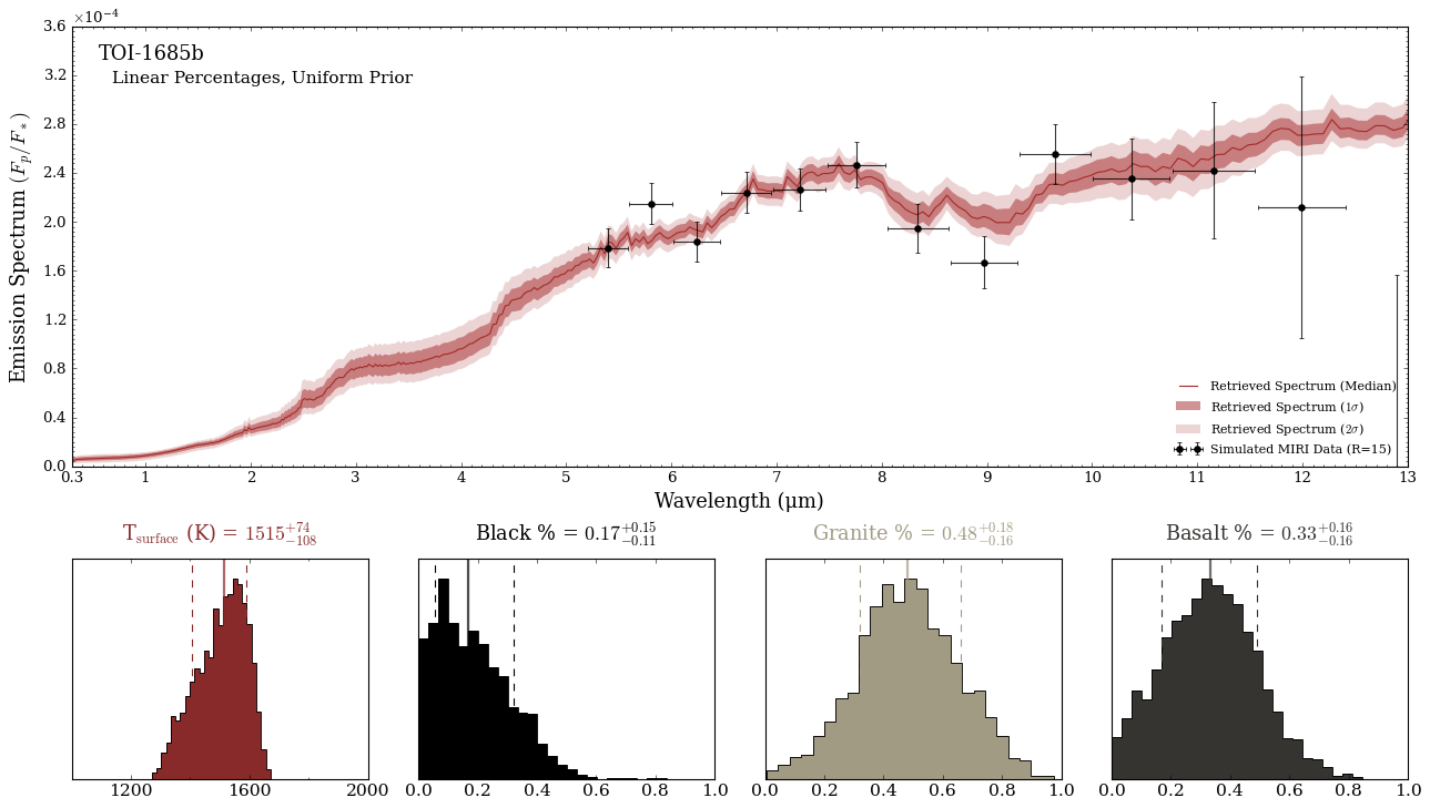
Plotting Emission Retrieval Results
Thats pretty fast! This is because for bare rocks, we don’t have to propogate radiation throughout a pesky atmosphere.
Lets go ahead and plot the results
Note that for emission retrievals, POSEIDON saves Fp (not Fp/Fs), and therefore we must convert the retrieved spectra ourselves to Fp/Fs space.
[11]:
#***** Plotting magic *****#

import matplotlib.pyplot as plt
from POSEIDON.visuals import plot_histograms

fig_combined = plt.figure(constrained_layout=True, figsize=(16,9))    # Change (9,5.5) to alter the aspect ratio

# This function is the magic. Each letter corresponds to one matplotlib axis, which you can then pass to POSEIDON's plotting functions
axd = fig_combined.subplot_mosaic(
    """
    AAAA
    AAAA
    abcd
    """
)

# Read retrieved spectrum confidence regions
wl, spec_low2, spec_low1, spec_median, \
spec_high1, spec_high2 = read_retrieved_spectrum(planet_name, model_name_linear_uniform)

# Convert to Fp/Fs
d = 1        # This value only used for flux ratios, so it cancels

# Load stellar spectrum
F_s = star['F_star']
R_s = star['R_s']

# Convert stellar surface flux to observed flux at Earth
F_s_obs = (R_s / d)**2 * F_s

spec_low2 = spec_low2 / F_s_obs
spec_low1 = spec_low1 / F_s_obs
spec_median = spec_median / F_s_obs
spec_high1 = spec_high1 / F_s_obs
spec_high2 = spec_high2 / F_s_obs

# Plot
# Create composite spectra objects for plotting
spectra_median = plot_collection(spec_median, wl, collection = [])
spectra_low1 = plot_collection(spec_low1, wl, collection = [])
spectra_low2 = plot_collection(spec_low2, wl, collection = [])
spectra_high1 = plot_collection(spec_high1, wl, collection = [])
spectra_high2 = plot_collection(spec_high2, wl, collection = [])

# Produce figure
ax_spectrum = axd['A']
_ = plot_spectra_retrieved(spectra_median, spectra_low2, spectra_low1,
                        spectra_high1, spectra_high2, planet_name,
                        data, R_to_bin = 150, show_ymodel = False,
                        colour_list = ['brown'],
                        spectra_labels = ['Retrieved Spectrum'],
                        plt_label = 'Linear Percentages, Uniform Prior',
                        figure_shape = 'wide', save_fig = False,
                        ax = ax_spectrum,
                        sigma_to_plot = 2,
                        y_unit = 'eclipse_depth',
                        legend_location = 'lower right',
                        wl_axis = 'linear',
                        data_marker_size_list = [5],
                        data_colour_list = ['black'],
                        y_min = 0, y_max = 3.6e-4,
                        data_labels = ['Simulated MIRI Data (R=15)'],
                        wl_max = 13,
                        line_alpha_list = [1]
                        )

# Plot histograms
axes_histograms = [axd["a"],axd["b"],axd["c"],axd["d"]]

models = [model_linear_uniform]

_ = plot_histograms(planet, models, plot_parameters = ['T_surf','Black_percentage',
                                                       'Granitoid_H12_percentage',
                                                       'Tholeiitic_basalt_H25_percentage'],
                    span = ((1000,2000),(0,1),(0,1),(0,1)),
                    N_bins = [25,25,25,25],
                    parameter_colour_list = ["#892a2a",'black','#a29b84',"#363431"],
                    axes = axes_histograms, save_fig = False,
                    tick_labelsize = 14,                          # x axis tick labels
                    title_fontsize = 16,                          # Title size
                    alpha_hist = [1,1,1,1],
                    title_alpha_list = [1,1,1,1],
                    custom_labels = ['T$_\mathrm{surface}$ (K)', 'Black %','Granite %','Basalt %'],
                    title_vert_spacing = 0.2,
                    title_colour_list = ["#892a2a",'black','#a29b84',"#363431"],
                    )
<Figure size 853.36x480 with 0 Axes>
<Figure size 600x400 with 0 Axes>
It looks like we have some mid-infrared feature around 8-9 microns! We can see how granite is the highest percentage, but that the forward model can produce degeneracies by combining the three albedo spectra together.
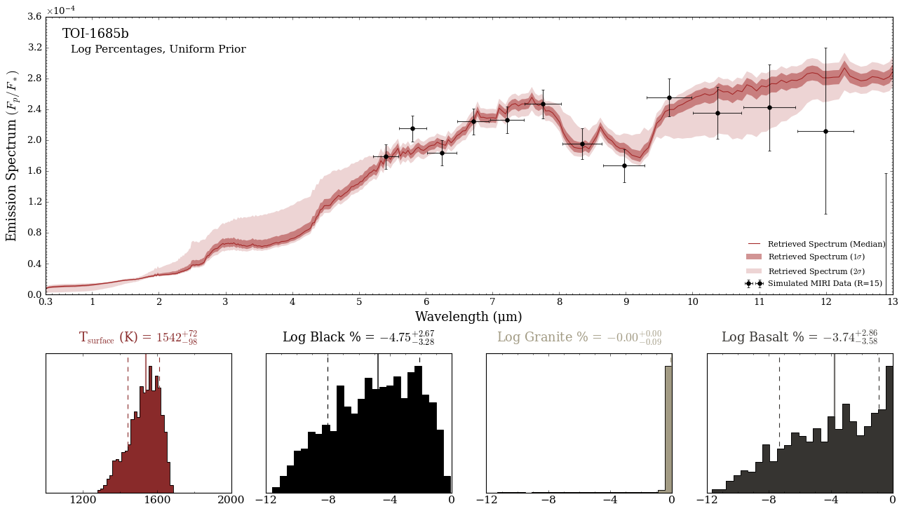
Uniform Prior, Log Percentages
[ ]:
# Initialise prior type dictionary
prior_types = {}

# Specify uniform priors for all free parameters
prior_types['R_p_ref'] = 'uniform'
prior_types['T_surf'] = 'uniform'

prior_types['log_Black_percentage'] = 'uniform'
prior_types['log_Granitoid_H12_percentage'] = 'uniform'
prior_types['log_Tholeiitic_basalt_H25_percentage'] = 'uniform'

# Initialise prior range dictionary
prior_ranges = {}

# Specify prior ranges for each free parameter
prior_ranges['R_p_ref'] = [0.9*R_p, 1.1*R_p]

prior_ranges['T_surf'] = [100,2000]

# Now, since its log 10 percentage, we do 1e-12 to 0
prior_ranges['log_Black_percentage'] = [-12,0]
prior_ranges['log_Granitoid_H12_percentage'] = [-12,0]
prior_ranges['log_Tholeiitic_basalt_H25_percentage'] = [-12,0]

# Create prior object for retrieval
priors = set_priors(planet, star, model_log_uniform, data, prior_types, prior_ranges)
[ ]:
#***** Specify fixed atmospheric settings for retrieval *****#

P = []
P_ref = []
opac = []

# We redefine the model wavelength grid and star just for convenience in the Jupyter notebook (in case cells are run out of order)

#***** Model wavelength grid *****#

wl_min = 0.3     # Minimum wavelength (um)
wl_max = 15     # Maximum wavelength (um)
R = 1000         # Spectral resolution of grid

wl = wl_grid_constant_R(wl_min, wl_max,R)

#***** Define stellar properties *****#

R_s = 0.4555*R_Sun      # Stellar radius (m)
T_s = 3575        # Stellar effective temperature (K)
Met_s = 0.3          # Stellar metallicity [log10(Fe/H_star / Fe/H_solar)] <--- note: for PHOENIX, only the solar metallicity models are used
log_g_s = 4.778       # Stellar log surface gravity (log10(cm/s^2) by convention)

# Create the stellar object
star = create_star(R_s, T_s, log_g_s, Met_s, wl = wl, stellar_grid = 'phoenix')

run_retrieval(planet, star, model_log_uniform, opac, data, priors, wl, P, P_ref, R = R,
                spectrum_type = 'emission', sampling_algorithm = 'MultiNest',
                N_live = 500, verbose = True, resume = False)
POSEIDON now running 'TOI-1685b-Log-Percentages-Uniform'
*****************************************************
MultiNest v3.10
Copyright Farhan Feroz & Mike Hobson
Release Jul 2015
no. of live points = 500
dimensionality = 5
*****************************************************
Starting MultiNest
generating live points
live points generated, starting sampling
Acceptance Rate: 0.994575
Replacements: 550
Total Samples: 553
Nested Sampling ln(Z): -497.290081
Acceptance Rate: 0.978793
Replacements: 600
Total Samples: 613
Nested Sampling ln(Z): -464.367428
Acceptance Rate: 0.948905
Replacements: 650
Total Samples: 685
Nested Sampling ln(Z): -408.026753
Acceptance Rate: 0.930851
Replacements: 700
Total Samples: 752
Nested Sampling ln(Z): -325.612091
Acceptance Rate: 0.915751
Replacements: 750
Total Samples: 819
Nested Sampling ln(Z): -217.984041
Acceptance Rate: 0.893855
Replacements: 800
Total Samples: 895
Nested Sampling ln(Z): -163.650959
Acceptance Rate: 0.886340
Replacements: 850
Total Samples: 959
Nested Sampling ln(Z): -107.132191
Acceptance Rate: 0.881489
Replacements: 900
Total Samples: 1021
Nested Sampling ln(Z): -73.647208
Acceptance Rate: 0.870761
Replacements: 950
Total Samples: 1091
Nested Sampling ln(Z): -33.658462
Acceptance Rate: 0.858369
Replacements: 1000
Total Samples: 1165
Nested Sampling ln(Z): -4.718458
Acceptance Rate: 0.846774
Replacements: 1050
Total Samples: 1240
Nested Sampling ln(Z): 14.942105
Acceptance Rate: 0.837776
Replacements: 1100
Total Samples: 1313
Nested Sampling ln(Z): 32.554890
Acceptance Rate: 0.833938
Replacements: 1150
Total Samples: 1379
Nested Sampling ln(Z): 47.370113
Acceptance Rate: 0.826446
Replacements: 1200
Total Samples: 1452
Nested Sampling ln(Z): 60.310144
Acceptance Rate: 0.815927
Replacements: 1250
Total Samples: 1532
Nested Sampling ln(Z): 69.199596
Acceptance Rate: 0.809465
Replacements: 1300
Total Samples: 1606
Nested Sampling ln(Z): 78.649121
Acceptance Rate: 0.800712
Replacements: 1350
Total Samples: 1686
Nested Sampling ln(Z): 85.258672
Acceptance Rate: 0.796813
Replacements: 1400
Total Samples: 1757
Nested Sampling ln(Z): 90.586589
Acceptance Rate: 0.792350
Replacements: 1450
Total Samples: 1830
Nested Sampling ln(Z): 94.542451
Acceptance Rate: 0.791139
Replacements: 1500
Total Samples: 1896
Nested Sampling ln(Z): 98.285131
Acceptance Rate: 0.784413
Replacements: 1550
Total Samples: 1976
Nested Sampling ln(Z): 102.426136
Acceptance Rate: 0.775194
Replacements: 1600
Total Samples: 2064
Nested Sampling ln(Z): 104.744664
Acceptance Rate: 0.768872
Replacements: 1650
Total Samples: 2146
Nested Sampling ln(Z): 106.570850
Acceptance Rate: 0.763016
Replacements: 1700
Total Samples: 2228
Nested Sampling ln(Z): 107.955014
Acceptance Rate: 0.757576
Replacements: 1750
Total Samples: 2310
Nested Sampling ln(Z): 109.187412
Acceptance Rate: 0.753769
Replacements: 1800
Total Samples: 2388
Nested Sampling ln(Z): 110.255889
Acceptance Rate: 0.748988
Replacements: 1850
Total Samples: 2470
Nested Sampling ln(Z): 111.317092
Acceptance Rate: 0.739012
Replacements: 1900
Total Samples: 2571
Nested Sampling ln(Z): 112.267070
Acceptance Rate: 0.731707
Replacements: 1950
Total Samples: 2665
Nested Sampling ln(Z): 113.136777
Acceptance Rate: 0.728597
Replacements: 2000
Total Samples: 2745
Nested Sampling ln(Z): 113.954385
Acceptance Rate: 0.725921
Replacements: 2050
Total Samples: 2824
Nested Sampling ln(Z): 114.668223
Acceptance Rate: 0.723140
Replacements: 2100
Total Samples: 2904
Nested Sampling ln(Z): 115.287082
Acceptance Rate: 0.713575
Replacements: 2150
Total Samples: 3013
Nested Sampling ln(Z): 115.768089
Acceptance Rate: 0.708763
Replacements: 2200
Total Samples: 3104
Nested Sampling ln(Z): 116.173126
Acceptance Rate: 0.703785
Replacements: 2250
Total Samples: 3197
Nested Sampling ln(Z): 116.510841
Acceptance Rate: 0.700579
Replacements: 2300
Total Samples: 3283
Nested Sampling ln(Z): 116.781945
Acceptance Rate: 0.695884
Replacements: 2350
Total Samples: 3377
Nested Sampling ln(Z): 117.008291
Acceptance Rate: 0.691842
Replacements: 2400
Total Samples: 3469
Nested Sampling ln(Z): 117.204145
Acceptance Rate: 0.685506
Replacements: 2450
Total Samples: 3574
Nested Sampling ln(Z): 117.410263
Acceptance Rate: 0.681570
Replacements: 2500
Total Samples: 3668
Nested Sampling ln(Z): 117.622027
Acceptance Rate: 0.678733
Replacements: 2550
Total Samples: 3757
Nested Sampling ln(Z): 117.816309
Acceptance Rate: 0.673052
Replacements: 2600
Total Samples: 3863
Nested Sampling ln(Z): 117.996285
Acceptance Rate: 0.668854
Replacements: 2650
Total Samples: 3962
Nested Sampling ln(Z): 118.166624
Acceptance Rate: 0.665680
Replacements: 2700
Total Samples: 4056
Nested Sampling ln(Z): 118.319180
Acceptance Rate: 0.658998
Replacements: 2750
Total Samples: 4173
Nested Sampling ln(Z): 118.453970
Acceptance Rate: 0.656045
Replacements: 2800
Total Samples: 4268
Nested Sampling ln(Z): 118.578945
Acceptance Rate: 0.653670
Replacements: 2850
Total Samples: 4360
Nested Sampling ln(Z): 118.695072
Acceptance Rate: 0.649787
Replacements: 2900
Total Samples: 4463
Nested Sampling ln(Z): 118.800485
Acceptance Rate: 0.644950
Replacements: 2950
Total Samples: 4574
Nested Sampling ln(Z): 118.895242
Acceptance Rate: 0.642949
Replacements: 3000
Total Samples: 4666
Nested Sampling ln(Z): 118.979136
Acceptance Rate: 0.639011
Replacements: 3050
Total Samples: 4773
Nested Sampling ln(Z): 119.055518
Acceptance Rate: 0.635897
Replacements: 3100
Total Samples: 4875
Nested Sampling ln(Z): 119.125844
Acceptance Rate: 0.635209
Replacements: 3150
Total Samples: 4959
Nested Sampling ln(Z): 119.189696
Acceptance Rate: 0.632536
Replacements: 3200
Total Samples: 5059
Nested Sampling ln(Z): 119.247825
Acceptance Rate: 0.628627
Replacements: 3250
Total Samples: 5170
Nested Sampling ln(Z): 119.300561
Acceptance Rate: 0.624054
Replacements: 3300
Total Samples: 5288
Nested Sampling ln(Z): 119.347996
Acceptance Rate: 0.619224
Replacements: 3350
Total Samples: 5410
Nested Sampling ln(Z): 119.391144
Acceptance Rate: 0.616836
Replacements: 3400
Total Samples: 5512
Nested Sampling ln(Z): 119.430202
Acceptance Rate: 0.614098
Replacements: 3450
Total Samples: 5618
Nested Sampling ln(Z): 119.465497
Acceptance Rate: 0.613045
Replacements: 3487
Total Samples: 5688
Nested Sampling ln(Z): 119.489617
POSEIDON retrieval finished in 0.0063 hours
ln(ev)= 119.81119829943626 +/- 8.7005552518691201E-002
Total Likelihood Evaluations: 5688
Sampling finished. Exiting MultiNest
Now generating 1000 sampled spectra and P-T profiles from the posterior distribution...
This process will take approximately 0.052 minutes
All done! Output files can be found in ./POSEIDON_output/TOI-1685b/retrievals/results/
[19]:
#***** Plotting magic *****#

import matplotlib.pyplot as plt
from POSEIDON.visuals import plot_histograms

fig_combined = plt.figure(constrained_layout=True, figsize=(16,9))    # Change (9,5.5) to alter the aspect ratio

# This function is the magic. Each letter corresponds to one matplotlib axis, which you can then pass to POSEIDON's plotting functions
axd = fig_combined.subplot_mosaic(
    """
    AAAA
    AAAA
    abcd
    """
)

# Read retrieved spectrum confidence regions
wl, spec_low2, spec_low1, spec_median, \
spec_high1, spec_high2 = read_retrieved_spectrum(planet_name, model_name_log_uniform)

# Convert to Fp/Fs
d = 1        # This value only used for flux ratios, so it cancels

# Load stellar spectrum
F_s = star['F_star']
R_s = star['R_s']

# Convert stellar surface flux to observed flux at Earth
F_s_obs = (R_s / d)**2 * F_s

spec_low2 = spec_low2 / F_s_obs
spec_low1 = spec_low1 / F_s_obs
spec_median = spec_median / F_s_obs
spec_high1 = spec_high1 / F_s_obs
spec_high2 = spec_high2 / F_s_obs

# Plot
# Create composite spectra objects for plotting
spectra_median = plot_collection(spec_median, wl, collection = [])
spectra_low1 = plot_collection(spec_low1, wl, collection = [])
spectra_low2 = plot_collection(spec_low2, wl, collection = [])
spectra_high1 = plot_collection(spec_high1, wl, collection = [])
spectra_high2 = plot_collection(spec_high2, wl, collection = [])

# Produce figure
ax_spectrum = axd['A']
_ = plot_spectra_retrieved(spectra_median, spectra_low2, spectra_low1,
                        spectra_high1, spectra_high2, planet_name,
                        data, R_to_bin = 150, show_ymodel = False,
                        colour_list = ['brown'],
                        spectra_labels = ['Retrieved Spectrum'],
                        plt_label = 'Log Percentages, Uniform Prior',
                        figure_shape = 'wide', save_fig = False,
                        ax = ax_spectrum,
                        sigma_to_plot = 2,
                        y_unit = 'eclipse_depth',
                        legend_location = 'lower right',
                        wl_axis = 'linear',
                        data_marker_size_list = [5],
                        data_colour_list = ['black'],
                        y_min = 0, y_max = 3.6e-4,
                        data_labels = ['Simulated MIRI Data (R=15)'],
                        wl_max = 13,
                        line_alpha_list = [1]
                        )

# Plot histograms
axes_histograms = [axd["a"],axd["b"],axd["c"],axd["d"]]

models = [model_log_uniform]

_ = plot_histograms(planet, models, plot_parameters = ['T_surf','log_Black_percentage',
                                                       'log_Granitoid_H12_percentage',
                                                       'log_Tholeiitic_basalt_H25_percentage'],
                    span = ((1000,2000),(-12,0),(-12,0),(-12,0)),
                    N_bins = [25,25,25,25],
                    parameter_colour_list = ["#892a2a",'black','#a29b84',"#363431"],
                    axes = axes_histograms, save_fig = False,
                    tick_labelsize = 14,                          # x axis tick labels
                    title_fontsize = 16,                          # Title size
                    alpha_hist = [1,1,1,1],
                    title_alpha_list = [1,1,1,1],
                    custom_labels = ['T$_\mathrm{surface}$ (K)', 'Log Black %','Log Granite %','Log Basalt %'],
                    title_vert_spacing = 0.2,
                    title_colour_list = ["#892a2a",'black','#a29b84',"#363431"],
                    )
<Figure size 853.36x480 with 0 Axes>
<Figure size 600x400 with 0 Axes>
In log space, it becomes a lot more obvious that granite is most likely to be the ‘bulk’ surface.
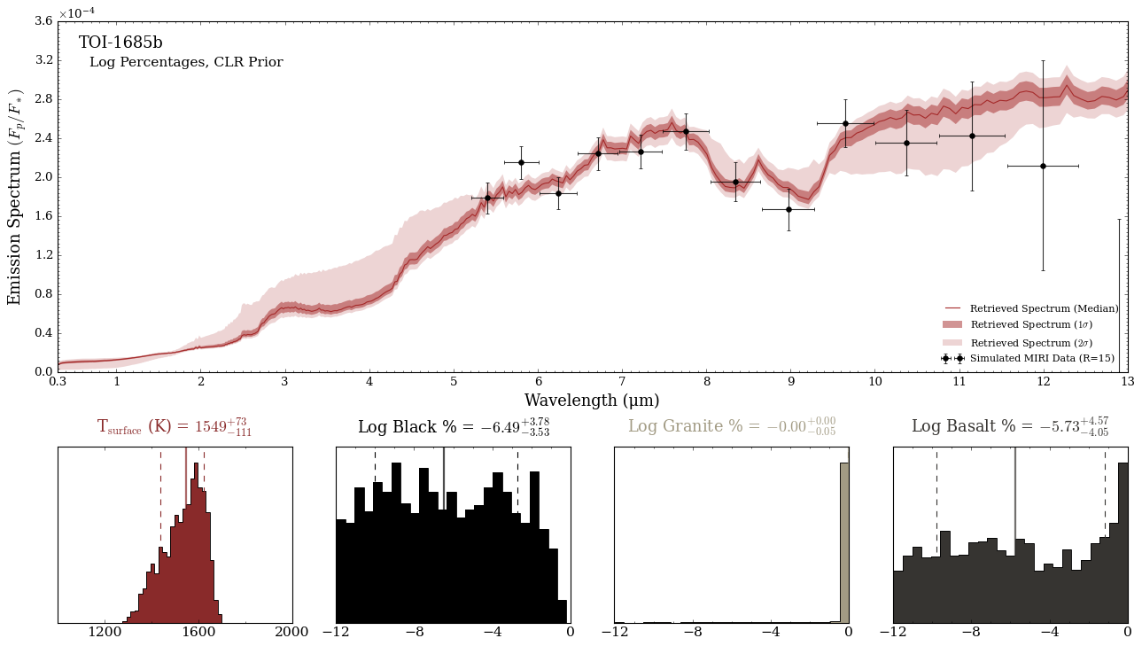
CLR Prior, Log Percentages
Here, we set the prior type to ‘CLR_surface’
The first surface component, ‘black’, will be the ‘fill’ surface (i.e., the non-free parameter that is added to granite + basalt to make the percentage 100%).
[15]:
# Initialise prior type dictionary
prior_types = {}

# Specify uniform priors for all free parameters
prior_types['R_p_ref'] = 'uniform'
prior_types['T_surf'] = 'uniform'

prior_types['log_Black_percentage'] = 'CLR_surface'
prior_types['log_Granitoid_H12_percentage'] = 'CLR_surface'
prior_types['log_Tholeiitic_basalt_H25_percentage'] = 'CLR_surface'

# Initialise prior range dictionary
prior_ranges = {}

# Specify prior ranges for each free parameter
prior_ranges['R_p_ref'] = [0.9*R_p, 1.1*R_p]

prior_ranges['T_surf'] = [100,2000]

prior_ranges['log_Black_percentage'] = [-12,0]
prior_ranges['log_Granitoid_H12_percentage'] = [-12,0]
prior_ranges['log_Tholeiitic_basalt_H25_percentage'] = [-12,0]

# Create prior object for retrieval
priors = set_priors(planet, star, model_log_clr, data, prior_types, prior_ranges)
[16]:
#***** Specify fixed atmospheric settings for retrieval *****#

P = []
P_ref = []
opac = []

#***** Model wavelength grid *****#

wl_min = 0.3     # Minimum wavelength (um)
wl_max = 15     # Maximum wavelength (um)
R = 1000         # Spectral resolution of grid

wl = wl_grid_constant_R(wl_min, wl_max,R)

#***** Define stellar properties *****#

R_s = 0.4555*R_Sun      # Stellar radius (m)
T_s = 3575        # Stellar effective temperature (K)
Met_s = 0.3          # Stellar metallicity [log10(Fe/H_star / Fe/H_solar)] <--- note: for PHOENIX, only the solar metallicity models are used
log_g_s = 4.778       # Stellar log surface gravity (log10(cm/s^2) by convention)

# Create the stellar object
star = create_star(R_s, T_s, log_g_s, Met_s, wl = wl, stellar_grid = 'phoenix')

run_retrieval(planet, star, model_log_clr, opac, data, priors, wl, P, P_ref, R = R,
                spectrum_type = 'emission', sampling_algorithm = 'MultiNest',
                N_live = 500, verbose = True, resume = False)
POSEIDON now running 'TOI-1685b-Log-Percentages-CLR'
*****************************************************
MultiNest v3.10
Copyright Farhan Feroz & Mike Hobson
Release Jul 2015
no. of live points = 500
dimensionality = 5
*****************************************************
Starting MultiNest
generating live points
live points generated, starting sampling
Acceptance Rate: 0.998185
Replacements: 550
Total Samples: 551
Nested Sampling ln(Z): -496.907870
Acceptance Rate: 0.993377
Replacements: 600
Total Samples: 604
Nested Sampling ln(Z): -473.018264
Acceptance Rate: 0.977444
Replacements: 650
Total Samples: 665
Nested Sampling ln(Z): -408.653354
Acceptance Rate: 0.953678
Replacements: 700
Total Samples: 734
Nested Sampling ln(Z): -338.723462
Acceptance Rate: 0.924784
Replacements: 750
Total Samples: 811
Nested Sampling ln(Z): -256.291887
Acceptance Rate: 0.897868
Replacements: 800
Total Samples: 891
Nested Sampling ln(Z): -195.659961
Acceptance Rate: 0.861196
Replacements: 850
Total Samples: 987
Nested Sampling ln(Z): -148.015015
Acceptance Rate: 0.845070
Replacements: 900
Total Samples: 1065
Nested Sampling ln(Z): -104.330046
Acceptance Rate: 0.823224
Replacements: 950
Total Samples: 1154
Nested Sampling ln(Z): -64.168163
Acceptance Rate: 0.802568
Replacements: 1000
Total Samples: 1246
Nested Sampling ln(Z): -33.734339
Acceptance Rate: 0.784753
Replacements: 1050
Total Samples: 1338
Nested Sampling ln(Z): -6.166869
Acceptance Rate: 0.771930
Replacements: 1100
Total Samples: 1425
Nested Sampling ln(Z): 13.530437
Acceptance Rate: 0.757077
Replacements: 1150
Total Samples: 1519
Nested Sampling ln(Z): 30.912013
Acceptance Rate: 0.730816
Replacements: 1200
Total Samples: 1642
Nested Sampling ln(Z): 43.217085
Acceptance Rate: 0.722961
Replacements: 1250
Total Samples: 1729
Nested Sampling ln(Z): 57.610068
Acceptance Rate: 0.711939
Replacements: 1300
Total Samples: 1826
Nested Sampling ln(Z): 67.002485
Acceptance Rate: 0.697314
Replacements: 1350
Total Samples: 1936
Nested Sampling ln(Z): 76.009742
Acceptance Rate: 0.688299
Replacements: 1400
Total Samples: 2034
Nested Sampling ln(Z): 81.163701
Acceptance Rate: 0.682032
Replacements: 1450
Total Samples: 2126
Nested Sampling ln(Z): 86.237929
Acceptance Rate: 0.676895
Replacements: 1500
Total Samples: 2216
Nested Sampling ln(Z): 91.912643
Acceptance Rate: 0.673328
Replacements: 1550
Total Samples: 2302
Nested Sampling ln(Z): 96.009663
Acceptance Rate: 0.669176
Replacements: 1600
Total Samples: 2391
Nested Sampling ln(Z): 99.282987
Acceptance Rate: 0.661058
Replacements: 1650
Total Samples: 2496
Nested Sampling ln(Z): 102.660150
Acceptance Rate: 0.654349
Replacements: 1700
Total Samples: 2598
Nested Sampling ln(Z): 105.055374
Acceptance Rate: 0.647908
Replacements: 1750
Total Samples: 2701
Nested Sampling ln(Z): 106.940995
Acceptance Rate: 0.644699
Replacements: 1800
Total Samples: 2792
Nested Sampling ln(Z): 108.343922
Acceptance Rate: 0.642584
Replacements: 1850
Total Samples: 2879
Nested Sampling ln(Z): 109.389434
Acceptance Rate: 0.638012
Replacements: 1900
Total Samples: 2978
Nested Sampling ln(Z): 110.222470
Acceptance Rate: 0.632706
Replacements: 1950
Total Samples: 3082
Nested Sampling ln(Z): 111.042736
Acceptance Rate: 0.631512
Replacements: 2000
Total Samples: 3167
Nested Sampling ln(Z): 111.868714
Acceptance Rate: 0.630381
Replacements: 2050
Total Samples: 3252
Nested Sampling ln(Z): 112.697638
Acceptance Rate: 0.628931
Replacements: 2100
Total Samples: 3339
Nested Sampling ln(Z): 113.570229
Acceptance Rate: 0.625728
Replacements: 2150
Total Samples: 3436
Nested Sampling ln(Z): 114.334800
Acceptance Rate: 0.625711
Replacements: 2200
Total Samples: 3516
Nested Sampling ln(Z): 114.954227
Acceptance Rate: 0.622751
Replacements: 2250
Total Samples: 3613
Nested Sampling ln(Z): 115.468008
Acceptance Rate: 0.617118
Replacements: 2300
Total Samples: 3727
Nested Sampling ln(Z): 115.907567
Acceptance Rate: 0.613577
Replacements: 2350
Total Samples: 3830
Nested Sampling ln(Z): 116.268601
Acceptance Rate: 0.609601
Replacements: 2400
Total Samples: 3937
Nested Sampling ln(Z): 116.555117
Acceptance Rate: 0.605387
Replacements: 2450
Total Samples: 4047
Nested Sampling ln(Z): 116.793411
Acceptance Rate: 0.600384
Replacements: 2500
Total Samples: 4164
Nested Sampling ln(Z): 117.002750
Acceptance Rate: 0.595516
Replacements: 2550
Total Samples: 4282
Nested Sampling ln(Z): 117.223113
Acceptance Rate: 0.593066
Replacements: 2600
Total Samples: 4384
Nested Sampling ln(Z): 117.442757
Acceptance Rate: 0.589151
Replacements: 2650
Total Samples: 4498
Nested Sampling ln(Z): 117.657374
Acceptance Rate: 0.585429
Replacements: 2700
Total Samples: 4612
Nested Sampling ln(Z): 117.849484
Acceptance Rate: 0.581764
Replacements: 2750
Total Samples: 4727
Nested Sampling ln(Z): 118.023829
Acceptance Rate: 0.578871
Replacements: 2800
Total Samples: 4837
Nested Sampling ln(Z): 118.180755
Acceptance Rate: 0.572749
Replacements: 2850
Total Samples: 4976
Nested Sampling ln(Z): 118.316998
Acceptance Rate: 0.569521
Replacements: 2900
Total Samples: 5092
Nested Sampling ln(Z): 118.439084
Acceptance Rate: 0.567526
Replacements: 2950
Total Samples: 5198
Nested Sampling ln(Z): 118.549499
Acceptance Rate: 0.563698
Replacements: 3000
Total Samples: 5322
Nested Sampling ln(Z): 118.649964
Acceptance Rate: 0.558199
Replacements: 3050
Total Samples: 5464
Nested Sampling ln(Z): 118.742595
Acceptance Rate: 0.553769
Replacements: 3100
Total Samples: 5598
Nested Sampling ln(Z): 118.826865
Acceptance Rate: 0.551954
Replacements: 3150
Total Samples: 5707
Nested Sampling ln(Z): 118.904039
Acceptance Rate: 0.549356
Replacements: 3200
Total Samples: 5825
Nested Sampling ln(Z): 118.973797
Acceptance Rate: 0.544024
Replacements: 3250
Total Samples: 5974
Nested Sampling ln(Z): 119.036283
Acceptance Rate: 0.542585
Replacements: 3300
Total Samples: 6082
Nested Sampling ln(Z): 119.092879
Acceptance Rate: 0.538326
Replacements: 3350
Total Samples: 6223
Nested Sampling ln(Z): 119.143941
Acceptance Rate: 0.538315
Replacements: 3400
Total Samples: 6316
Nested Sampling ln(Z): 119.190254
Acceptance Rate: 0.536714
Replacements: 3450
Total Samples: 6428
Nested Sampling ln(Z): 119.232367
Acceptance Rate: 0.533781
Replacements: 3500
Total Samples: 6557
Nested Sampling ln(Z): 119.270761
Acceptance Rate: 0.531995
Replacements: 3550
Total Samples: 6673
Nested Sampling ln(Z): 119.305966
Acceptance Rate: 0.528405
Replacements: 3581
Total Samples: 6777
Nested Sampling ln(Z): 119.326292
POSEIDON retrieval finished in 0.0076 hours
ln(ev)= 119.65087682520353 +/- 8.9294505223800461E-002
Total Likelihood Evaluations: 6777
Sampling finished. Exiting MultiNest
Now generating 1000 sampled spectra and P-T profiles from the posterior distribution...
This process will take approximately 0.052 minutes
All done! Output files can be found in ./POSEIDON_output/TOI-1685b/retrievals/results/
[20]:
#***** Plotting magic *****#

import matplotlib.pyplot as plt
from POSEIDON.visuals import plot_histograms

fig_combined = plt.figure(constrained_layout=True, figsize=(16,9))    # Change (9,5.5) to alter the aspect ratio

# This function is the magic. Each letter corresponds to one matplotlib axis, which you can then pass to POSEIDON's plotting functions
axd = fig_combined.subplot_mosaic(
    """
    AAAA
    AAAA
    abcd
    """
)

# Read retrieved spectrum confidence regions
wl, spec_low2, spec_low1, spec_median, \
spec_high1, spec_high2 = read_retrieved_spectrum(planet_name, model_name_log_clr)

# Convert to Fp/Fs
d = 1        # This value only used for flux ratios, so it cancels

# Load stellar spectrum
F_s = star['F_star']
R_s = star['R_s']

# Convert stellar surface flux to observed flux at Earth
F_s_obs = (R_s / d)**2 * F_s

spec_low2 = spec_low2 / F_s_obs
spec_low1 = spec_low1 / F_s_obs
spec_median = spec_median / F_s_obs
spec_high1 = spec_high1 / F_s_obs
spec_high2 = spec_high2 / F_s_obs

# Plot
# Create composite spectra objects for plotting
spectra_median = plot_collection(spec_median, wl, collection = [])
spectra_low1 = plot_collection(spec_low1, wl, collection = [])
spectra_low2 = plot_collection(spec_low2, wl, collection = [])
spectra_high1 = plot_collection(spec_high1, wl, collection = [])
spectra_high2 = plot_collection(spec_high2, wl, collection = [])

# Produce figure
ax_spectrum = axd['A']
_ = plot_spectra_retrieved(spectra_median, spectra_low2, spectra_low1,
                        spectra_high1, spectra_high2, planet_name,
                        data, R_to_bin = 150, show_ymodel = False,
                        colour_list = ['brown'],
                        spectra_labels = ['Retrieved Spectrum'],
                        plt_label = 'Log Percentages, CLR Prior',
                        figure_shape = 'wide', save_fig = False,
                        ax = ax_spectrum,
                        sigma_to_plot = 2,
                        y_unit = 'eclipse_depth',
                        legend_location = 'lower right',
                        wl_axis = 'linear',
                        data_marker_size_list = [5],
                        data_colour_list = ['black'],
                        y_min = 0, y_max = 3.6e-4,
                        data_labels = ['Simulated MIRI Data (R=15)'],
                        wl_max = 13,
                        line_alpha_list = [1]
                        )

# Plot histograms
axes_histograms = [axd["a"],axd["b"],axd["c"],axd["d"]]

models = [model_log_clr]

_ = plot_histograms(planet, models, plot_parameters = ['T_surf','log_Black_percentage',
                                                       'log_Granitoid_H12_percentage',
                                                       'log_Tholeiitic_basalt_H25_percentage'],
                    span = ((1000,2000),(-12,0),(-12,0),(-12,0)),
                    N_bins = [25,25,25,25],
                    parameter_colour_list = ["#892a2a",'black','#a29b84',"#363431"],
                    axes = axes_histograms, save_fig = False,
                    tick_labelsize = 14,                          # x axis tick labels
                    title_fontsize = 16,                          # Title size
                    alpha_hist = [1,1,1,1],
                    title_alpha_list = [1,1,1,1],
                    custom_labels = ['T$_\mathrm{surface}$ (K)', 'Log Black %','Log Granite %','Log Basalt %'],
                    title_vert_spacing = 0.2,
                    title_colour_list = ["#892a2a",'black','#a29b84',"#363431"],
                    )
<Figure size 853.36x480 with 0 Axes>
<Figure size 600x400 with 0 Axes>
There we go! Looks like granite is the most likely surface component of this planet due to its strong feature at 8-9 microns (which is indicative of the mineral quartz), whereas basalt has a broader feature that is disfavored by the simualted data. Indeed, the data above was made from a forward model where granite was assumed to be 100% of the surface of this planet.
From here-on, one can perform retrievals with just a single surface component and compare bayesian evidences to see if we are truly detecting a singular surface component, or one can explore what the absorption feature would look like if the planet’s surface was a combination of 50% granite and 50% basalt.
If this was for a JWST proposal, once could explore adding on existing datasets (i.e., the recently published G395H eclipse dataset for this planet) to see if helps constrain the surface in conjunction with the MIRI data, or test whether or not you would need more MIRI transits to confidently detect granite, basalt, or a mix of the two.
Either way, JWST provides the unique mid-infrared capability to begin explore exo-geology on exoplanet surfaces.