High-Resolution Emission Retrievals
This tutorial covers how to run a retrieval with high-resolution ground-based emission data using POSEIDON.
Before you run this notebook, you should run the “Ground-Based High-Resolution Emission Spectroscopy (Cross Correlation)” tutorial first to preprocess the data. If you have data_processed.hdf5 saved in your planet directory, you are all set!
We will reproduce the result from Brogi and Line 2019, validating our framework on WASP-77Ab.
Loading WASP-77Ab Emission Data
First, we will load the processed data for WASP-77 Ab. For more information about this dataset and to learn the basics of high-resolution cross correlation spectroscopy, see the “Ground-Based High-Resolution Emission Spectroscopy (Cross Correlation)” tutorial.
[ ]:
from POSEIDON.high_res import read_high_res_data

planet_name = 'WASP-77Ab'

data_dir = '../../../POSEIDON/reference_data/observations/' + planet_name # The directory where you've put the data

data = read_high_res_data(data_dir, names=["IGRINS"])  # We named the dataset IGRINS in the previous notebook
Creating a Retrieval Model
Now, let’s provide the wavelength grid and properties of the host star and your planet. The wavelength range should match the range of your data, which spans 1.3 microns to 2.6 microns in this case.
We use R=250,000 as a tradeoff between computational speed and accuracy. For more discussion, see the previous tutorial.
[1]:
from POSEIDON.core import define_model, wl_grid_constant_R
from POSEIDON.core import create_star, create_planet
from POSEIDON.constants import R_Sun, R_J, M_J

# ***** Wavelength grid *****#

wl_min = 1.3  # Minimum wavelength (um)
wl_max = 2.6  # Maximum wavelength (um)
R = 250000    # Change the spectral resolution of grid here.

# Create a wavelength grid with constant R
wl = wl_grid_constant_R(wl_min, wl_max, R)

# ***** Define stellar properties *****#

R_s = 0.91 * R_Sun  # Stellar radius (m)
T_s = 5605.0        # Stellar effective temperature (K)
Met_s = -0.04       # Stellar metallicity [log10(Fe/H_star / Fe/H_solar)]
log_g_s = 4.48      # Stellar log surface gravity (log10(cm/s^2) by convention)

star = create_star(R_s, T_s, log_g_s, Met_s, wl=wl, stellar_grid="phoenix")

# ***** Define planet properties *****#

planet_name = "WASP-77Ab"  # Planet name used for plots, output files etc.

R_p = 1.21 * R_J  # Planetary radius (m)
M_p = 1.76 * M_J  # Mass of planet (kg)

# Create the planet object
planet = create_planet(planet_name, R_p, mass=M_p)

# If distance not specified, use fiducial value
if planet["system_distance"] is None:
    planet["system_distance"] = 1  # This value only used for flux ratios, so it cancels
d = planet["system_distance"]
Existing literature have shown detection of \(\rm{H}_2\rm{O}\), \(\rm{C}\rm{O}\), \(\rm{N}\rm{H}_3\), and \(\rm{C}\rm{H}_4\) in the atmosphere of WASP-77Ab.
So for a first attempt, we consider a model with \(\rm{H}_2\rm{O}\), \(\rm{C}\rm{O}\), \(\rm{N}\rm{H}_3\), and \(\rm{C}\rm{H}_4\), a 5-parameter temperature profile (Madhusudan & Seager 2009), and no clouds.
For additional parameters used in high resolution retrieval, we include: \(log_\alpha\) (the scaling parameter), \(K_p\) (the Keplerian orbital velocity), \(V_{sys}\) (the systematic velocity), and \(W_{conv}\) (width of the gaussian convolution kernel used for line broadening). An additional parameter available is \(\Delta \phi\) (offseting the ephemeris).
[2]:
# ***** Define model *****#

model_name = "Retrieval"  # Model name used for plots, output files etc.
bulk_species = ["H2", "He"]  # H2 + He comprises the bulk atmosphere

param_species = ["H2O", "CO", "NH3", "CH4"]

model = define_model(model_name, bulk_species, param_species,
                     PT_profile = "Madhu", reference_parameter = "R_p_ref",
                     high_res_method = "sysrem", # Important! Should be the same as the method used to preprocess the data
                     alpha_high_res_option = 'log',
                     fix_alpha_high_res = False, fix_W_conv_high_res = False,
                     fix_beta_high_res = True, fix_Delta_phi_high_res = True,
                     )

# Check the free parameters defining this model
print("Free parameters: " + str(model["param_names"]))
Free parameters: ['R_p_ref' 'a1' 'a2' 'log_P1' 'log_P2' 'log_P3' 'T_ref' 'log_H2O' 'log_CO'
 'log_NH3' 'log_CH4' 'K_p' 'V_sys' 'W_conv' 'log_alpha_HR']
Setting Retrieval Priors
One of the most important aspects in any Bayesian analysis is deciding what priors to use for the free parameters. Specifying a prior has two steps: (i) choosing the type of probability distribution; and (ii) choosing the allowable range.
Most free parameters in atmospheric retrievals with POSEIDON use the following prior types:
Uniform: you provide the minimum and maximum values for the parameter.
Gaussian: you provide the mean and standard deviation for the parameter.
Note:
If you do not specify a prior type or range for a given parameter, POSEIDON will ascribe a default prior type (generally uniform) and a ‘generous’ range.
This retrieval is defined by 15 free parameters printed above: (1) the radius at the (fixed) reference pressure; (2) the P-T profile parameters; (3) the log-mixing ratios; and (4) the four high resolution parameters.
Since we are assuming no a priori information on WASP-77Ab’s atmosphere, we will use uniform priors for all the parameters.
[4]:
from POSEIDON.core import set_priors

# ***** Set priors for retrieval *****#

# Initialise prior type dictionary
prior_types = {}

# Specify whether priors are linear, Gaussian, etc.
prior_types["T_ref"] = "uniform"
prior_types["R_p_ref"] = "uniform"
prior_types["log_X"] = "uniform"
prior_types["a1"] = "uniform"
prior_types["a2"] = "uniform"
prior_types["log_P1"] = "uniform"
prior_types["log_P2"] = "uniform"
prior_types["log_P3"] = "uniform"
prior_types["K_p"] = "uniform"
prior_types["V_sys"] = "uniform"
prior_types["log_alpha_HR"] = "uniform"
prior_types["W_conv"] = "uniform"

# Initialise prior range dictionary
prior_ranges = {}

# Specify prior ranges for each free parameter
prior_ranges["T_ref"] = [500, 2000]
prior_ranges["R_p_ref"] = [0.5 * R_p, 1.5 * R_p]
prior_ranges["log_X"] = [-15, 0]
prior_ranges["a1"] = [0, 1]
prior_ranges["a2"] = [0, 1]
prior_ranges["log_P1"] = [-5, 2]
prior_ranges["log_P2"] = [-5, 2]
prior_ranges["log_P3"] = [-2, 2]
prior_ranges["K_p"] = [150, 250]
prior_ranges["V_sys"] = [-50, 50]
prior_ranges["log_alpha_HR"] = [-2, 2]
prior_ranges["W_conv"] = [0, 50]

# Create prior object for retrieval
priors = set_priors(planet, star, model, data, prior_types, prior_ranges)
Pre-load Opacities
The last step before running a retrieval is to pre-interpolate the cross sections for our model and store them in memory. For more details on this process, see the forward model tutorial.
Warning:
Ensure the range of \(T_{\rm{fine}}\) used for opacity pre-interpolation is at least as large as the desired prior range for temperatures to be explored in the retrieval. Any models with layer temperatures falling outside the range of \(T_{\rm{fine}}\) will be automatically rejected (for retrievals with non-isothermal P-T profiles, this prevents unphysical profiles with negative temperatures etc.)
[ ]:
from POSEIDON.core import read_opacities
import numpy as np

# ***** Read opacity data *****#
opacity_treatment = "opacity_sampling"

# Define fine temperature grid (K)
T_fine_min = 400  # 400 K lower limit suffices for a typical hot Jupiter
T_fine_max = 4000  # 2000 K upper limit suffices for a typical hot Jupiter
T_fine_step = 50  # 20 K steps are a good tradeoff between accuracy and RAM

T_fine = np.arange(T_fine_min, (T_fine_max + T_fine_step), T_fine_step)

# Define fine pressure grid (log10(P/bar))
log_P_fine_min = -5.0  # 1 ubar is the lowest pressure in the opacity database
log_P_fine_max = 2  # 100 bar is the highest pressure in the opacity database
log_P_fine_step = 0.2  # 0.2 dex steps are a good tradeoff between accuracy and RAM

log_P_fine = np.arange(log_P_fine_min, (log_P_fine_max + log_P_fine_step), log_P_fine_step)

opac = read_opacities(model, wl, opacity_treatment, T_fine, log_P_fine)
Reading in cross sections in opacity sampling mode...
H2-H2 done
H2-He done
H2O done
CO done
Opacity pre-interpolation complete.
Run Retrieval
You are now ready to run your high resolution atmospheric retrieval on this dataset!
Tip:
Retrievals run faster on multiple cores. When running the cells in this Jupyter notebook, only a single core will be used. You can run a multi-core retrieval on 24 cores by converting this Jupyter notebook into a python script, then calling mpirun on the .py file:
mpirun -n 24 python -u YOUR_RETRIEVAL_SCRIPT.py
Important Note: A high resolution forward model is computationally expensive (~1 second per model). With 400 live points, it took > \(10^6\) evaluations for the model to converge. This retrieval could be finished with ~8 hours on 24 cores.
Instead of waiting until the end of time for the next cell to finish, you could run the ‘emission_high_res_retrieval.py’ file in this folder, which is the same code converted from this notebook, and parallelise with multiple cores in command line.
To check the code is working before launching a high-res retrieval, you can run the cell below and wait for a couple of minutes. Once it says “live points generated” and still no error, you are good to run it on multiple cores!
[ ]:
from POSEIDON.retrieval import run_retrieval

# ***** Specify fixed atmospheric settings for retrieval *****#

# Atmospheric pressure grid
P_min = 1e-5     # 10 ubar
P_max = 100     # 100 bar
N_layers = 100  # 100 layers

# Let's space the layers uniformly in log-pressure
P = np.logspace(np.log10(P_max), np.log10(P_min), N_layers)

# Specify the reference pressure and radius
P_ref = 1e-2  # Reference pressure (bar)

# ***** Run atmospheric retrieval *****#

run_retrieval(planet, star, model, opac, data, priors, wl, P, P_ref, R_p_ref = R_p,
              R = R, spectrum_type = "emission", sampling_algorithm = "MultiNest",
              N_live = 400, verbose = True, N_output_samples = 1000,
              resume = False)
POSEIDON now running 'Retrieval'
 *****************************************************
 MultiNest v3.10
 Copyright Farhan Feroz & Mike Hobson
 Release Jul 2015

 no. of live points =  400
 dimensionality =   13
 *****************************************************
 Starting MultiNest
 generating live points
 live points generated, starting sampling
Acceptance Rate:                        0.993377
Replacements:                                450
Total Samples:                               453
Nested Sampling ln(Z):            8309213.271610
Acceptance Rate:                        0.976562
Replacements:                                500
Total Samples:                               512
Nested Sampling ln(Z):            8309219.101900
Acceptance Rate:                        0.929054
Replacements:                                550
Total Samples:                               592
Nested Sampling ln(Z):            8309220.009087
Plot Retrieval Results
[ ]:
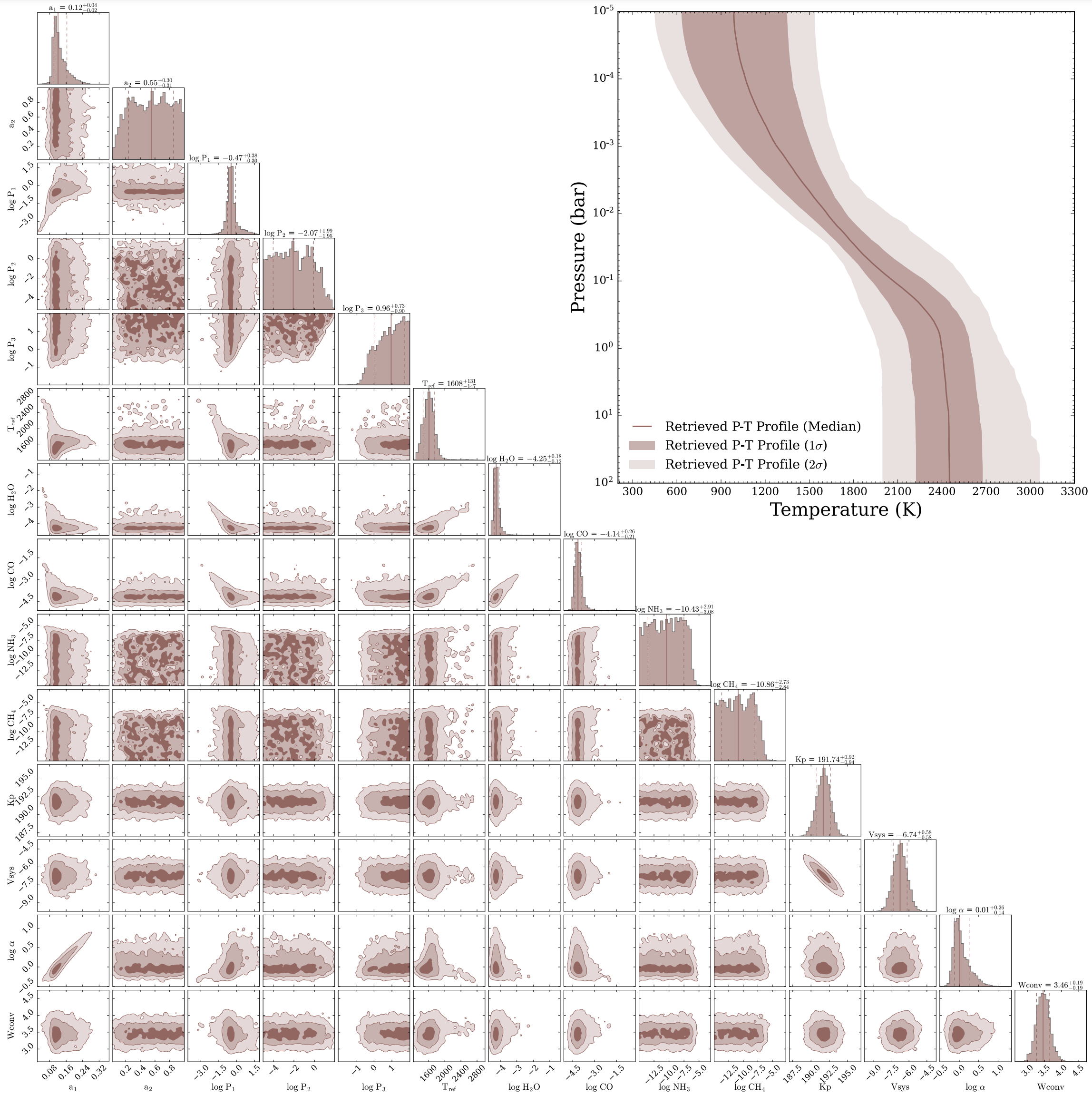
# Generate a corner plot after the retrieval is finished
from POSEIDON.corner import generate_cornerplot

fig_corner = generate_cornerplot(planet, model)
[ ]:
# Read retrieved PT profile and plot it
from POSEIDON.utility import read_retrieved_PT
from POSEIDON.visuals import plot_PT_retrieved

# Read the retrieved PT profile
P, T_low2, T_low1, T_median, \
T_high1, T_high2 = read_retrieved_PT(planet_name, model_name)


PT_median = [(T_median, P)]
PT_low2 = [(T_low2, P)]
PT_low1 = [(T_low1, P)]
PT_high1 = [(T_high1, P)]
PT_high2 = [(T_high2, P)]

# Plot the retrieved PT profile
plot_PT_retrieved(planet_name, PT_median, PT_low2, PT_low1, PT_high1, PT_high2,
                  # T_true=None, # Uncomment this line if you have a PT profile to compare to
                  # # colour_list=[], # Uncomment this line if you want to specify colors
                  T_min=2000, T_max=4000,
                  legend_location="lower left"
                  )
Below is the corner plot and retrieved PT profile from a retrieval on this dataset.