Atmospheric Retrievals with POSEIDON
At long last, your proposal to observe the newly discovered hot Jupiter WASP-999b with the Hubble Space Telescope has been accepted. Congratulations!
Loading Data
Months later, after carefully reducing the observations, you are ready to gaze in awe at your transmission spectrum.
First, you load all the usual stellar and planetary properties for this system.
[1]:
from POSEIDON.core import create_star, create_planet
from POSEIDON.constants import R_Sun, R_J

#***** Define stellar properties *****#

R_s = 1.155*R_Sun     # Stellar radius (m)
T_s = 6071.0          # Stellar effective temperature (K)
Met_s = 0.0           # Stellar metallicity [log10(Fe/H_star / Fe/H_solar)]
log_g_s = 4.38        # Stellar log surface gravity (log10(cm/s^2) by convention)

# Create the stellar object
star = create_star(R_s, T_s, log_g_s, Met_s)

#***** Define planet properties *****#

planet_name = 'WASP-999b'  # Planet name used for plots, output files etc.

R_p = 1.359*R_J     # Planetary radius (m)
g_p = 9.186         # Gravitational field of planet (m/s^2)
T_eq = 1400.0       # Equilibrium temperature (K)

# Create the planet object
planet = create_planet(planet_name, R_p, gravity = g_p, T_eq = T_eq)
Next, you plot your observed transmission spectrum of WASP-999b.
[2]:
from POSEIDON.core import load_data, wl_grid_constant_R
from POSEIDON.visuals import plot_data

#***** Model wavelength grid *****#

wl_min = 0.4      # Minimum wavelength (um)
wl_max = 3.0      # Maximum wavelength (um)
R = 4000         # Spectral resolution of grid

# We need to provide a model wavelength grid to initialise instrument properties
wl = wl_grid_constant_R(wl_min, wl_max, R)

#***** Specify data location and instruments  *****#

data_dir = '../../../POSEIDON/reference_data/observations/WASP-999b'         # Change this to where your data is stored
datasets = ['WASP-999b_WFC3_G141.dat']  # Found in reference_data/observations
instruments = ['WFC3_G141']             # Instruments corresponding to the data

# Load dataset, pre-load instrument PSF and transmission function
data = load_data(data_dir, datasets, instruments, wl)

# Plot our data
fig_data = plot_data(data, planet_name)
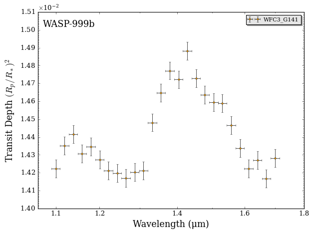
The spectrum isn’t flat! 🎉
Even better, your long term collaborator Dr. Tenalp just so happens to also have some observations of WASP-999b at shorter wavelengths. Let’s add their Hubble STIS data to our collection.
Note:
The data file format expected by POSEIDON is:
wavelength (μm) | bin half width (μm) | transit depth \((R_p/R_s)^2\) | transit depth error
[3]:
# Specify the STIS and WFC3 Hubble data
data_dir = '../../../POSEIDON/reference_data/observations/WASP-999b'
datasets = ['WASP-999b_STIS_G430.dat',
            'WASP-999b_STIS_G750.dat',
            'WASP-999b_WFC3_G141.dat']
instruments = ['STIS_G430', 'STIS_G750', 'WFC3_G141']

# Load dataset, pre-load instrument PSF and transmission function
data = load_data(data_dir, datasets, instruments, wl)

# Plot our data
fig_data = plot_data(data, planet_name)
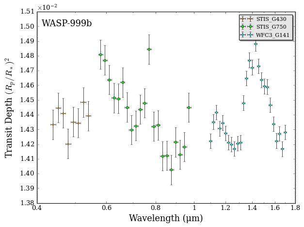
With data in hand, you are ready to begin the process of retrieving WASP-999b’s atmospheric properties.
Creating a Retrieval Model
Now comes the creative part: what model do you try first to fit WASP-999b’s transmission spectrum?
Given the a priori known low density of the planet, you conclude it is reasonable to assume this is a giant planet dominated by \(\rm{H}_2\) and \(\rm{He}\). Looking at your data above, especially the huge absorption feature in the infrared around 1.4 μm, you guess that \(\rm{H}_2 \rm{O}\) could be present (based on theoretical predictions or after looking up its cross section).
So for a first attempt, you consider a model with \(\rm{H}_2 \rm{O}\), an isothermal temperature profile, and no clouds.
[4]:
from POSEIDON.core import define_model

#***** Define model *****#

model_name = 'My_first_retrieval'  # Model name used for plots, output files etc.

bulk_species = ['H2', 'He']     # H2 + He comprises the bulk atmosphere
param_species = ['H2O']         # The only trace gas is H2O

# Create the model object
model = define_model(model_name, bulk_species, param_species,
                     PT_profile = 'isotherm', cloud_model = 'cloud-free')

# Check the free parameters defining this model
print("Free parameters: " + str(model['param_names']))
Free parameters: ['R_p_ref' 'T' 'log_H2O']
Setting Retrieval Priors
One of the most important aspects in any Bayesian analysis is deciding what priors to use for the free parameters. Specifying a prior has two steps: (i) choosing the type of probability distribution; and (ii) choosing the allowable range.
Most free parameters in atmospheric retrievals with POSEIDON use the following prior types:
Uniform: you provide the minimum and maximum values for the parameter.
Gaussian: you provide the mean and standard deviation for the parameter.
Note:
If you do not specify a prior type or range for a given parameter, POSEIDON will ascribe a default prior type (generally uniform) and a ‘generous’ range.
Priors for WASP-999b
Your first retrieval is defined by three free parameters: (1) the isothermal atmospheric temperature; (2) the radius at the (fixed) reference pressure; and (3) the log-mixing ratio of \(\rm{H}_2 \rm{O}\). Since you don’t have any a priori information on WASP-999b’s atmosphere, you decide to use uniform priors for the three parameters.
You think a reasonable prior range for the temperature of this hot Jupiter is \(400 \, \rm{K}\) to \((T_{\rm{eq}} + 200 \, \rm{K}) = 1600 \, \rm{K}\). For the reference radius, you choose a wide range from 85% to 115% of the observed white light radius. Finally, for the \(\rm{H}_2 \rm{O}\) abundance you ascribe a very broad range from \(10^{-12}\) to 0.1.
[5]:
from POSEIDON.core import set_priors

#***** Set priors for retrieval *****#

# Initialise prior type dictionary
prior_types = {}

# Specify whether priors are linear, Gaussian, etc.
prior_types['T'] = 'uniform'
prior_types['R_p_ref'] = 'uniform'
prior_types['log_H2O'] = 'uniform'

# Initialise prior range dictionary
prior_ranges = {}

# Specify prior ranges for each free parameter
prior_ranges['T'] = [400, 1600]
prior_ranges['R_p_ref'] = [0.85*R_p, 1.15*R_p]
prior_ranges['log_H2O'] = [-12, -1]

# Create prior object for retrieval
priors = set_priors(planet, star, model, data, prior_types, prior_ranges)
Pre-load Opacities
The last step before running a retrieval is to pre-interpolate the cross sections for our model and store them in memory. For more details on this process, see the forward model tutorial.
Warning:
Ensure the range of \(T_{\rm{fine}}\) used for opacity pre-interpolation is at least as large as the desired prior range for temperatures to be explored in the retrieval. Any models with layer temperatures falling outside the range of \(T_{\rm{fine}}\) will be automatically rejected (for retrievals with non-isothermal P-T profiles, this prevents unphysical profiles with negative temperatures etc.)
[6]:
from POSEIDON.core import read_opacities
import numpy as np

#***** Read opacity data *****#

opacity_treatment = 'opacity_sampling'

# Define fine temperature grid (K)
T_fine_min = 400     # Same as prior range for T
T_fine_max = 1600    # Same as prior range for T
T_fine_step = 10     # 10 K steps are a good tradeoff between accuracy and RAM

T_fine = np.arange(T_fine_min, (T_fine_max + T_fine_step), T_fine_step)

# Define fine pressure grid (log10(P/bar))
log_P_fine_min = -6.0   # 1 ubar is the lowest pressure in the opacity database
log_P_fine_max = 2.0    # 100 bar is the highest pressure in the opacity database
log_P_fine_step = 0.2   # 0.2 dex steps are a good tradeoff between accuracy and RAM

log_P_fine = np.arange(log_P_fine_min, (log_P_fine_max + log_P_fine_step),
                       log_P_fine_step)

# Pre-interpolate the opacities
opac = read_opacities(model, wl, opacity_treatment, T_fine, log_P_fine)
Reading in cross sections in opacity sampling mode...
H2-H2 done
H2-He done
H2O done
Opacity pre-interpolation complete.
Run Retrieval
You are now ready to run your first atmospheric retrieval!
Here we will use the nested sampling algorithm MultiNest to explore the parameter space. The key input quantity you need to provide to MultiNest is called the number of live points, \(N_{\rm{live}}\), which determines how finely the parameter space will be sampled (and hence the number of computed spectra). For exploratory retrievals, \(N_{\rm{live}} = 400\) usually suffices. For publication-quality results, \(N_{\rm{live}} = 2000\) is reasonable.
This simple POSEIDON retrieval should take about 10 minutes on 1 core for a typical laptop.
Tip:
Retrievals run faster on multiple cores. When running the cells in this Jupyter notebook, only a single core will be used. You can run a multi-core retrieval on 4 cores by converting this Jupyter notebook into a python script, then calling mpirun on the .py file:
mpirun -n 4 python -u YOUR_RETRIEVAL_SCRIPT.py
Note: If you are having issues with mpirun using more than the allotted number of cores, you can also try: mpirun -n 4 --bind-to core python -u YOUR_RETRIEVAL_SCRIPT.py In the same directory as this notebook, you’ll find the template file first_retrieval.py that you can look at for an example for a py script to run on multiple cores with.
[7]:
from POSEIDON.retrieval import run_retrieval

#***** Specify fixed atmospheric settings for retrieval *****#

# Atmospheric pressure grid
P_min = 1.0e-7    # 0.1 ubar
P_max = 100       # 100 bar
N_layers = 100    # 100 layers

# Let's space the layers uniformly in log-pressure
P = np.logspace(np.log10(P_max), np.log10(P_min), N_layers)

# Specify the reference pressure
P_ref = 10.0   # Retrieved R_p_ref parameter will be the radius at 10 bar

#***** Run atmospheric retrieval *****#

run_retrieval(planet, star, model, opac, data, priors, wl, P, P_ref, R = R,
              spectrum_type = 'transmission', sampling_algorithm = 'MultiNest',
              N_live = 400, verbose = True)
POSEIDON now running 'My_first_retrieval'
*****************************************************
MultiNest v3.10
Copyright Farhan Feroz & Mike Hobson
Release Jul 2015
no. of live points = 400
dimensionality = 3
*****************************************************
Starting MultiNest
generating live points
live points generated, starting sampling
Acceptance Rate: 0.980392
Replacements: 450
Total Samples: 459
Nested Sampling ln(Z): -134865.155519
Acceptance Rate: 0.956023
Replacements: 500
Total Samples: 523
Nested Sampling ln(Z): -75434.767207
Acceptance Rate: 0.929054
Replacements: 550
Total Samples: 592
Nested Sampling ln(Z): -61176.237528
Acceptance Rate: 0.891530
Replacements: 600
Total Samples: 673
Nested Sampling ln(Z): -46455.737724
Acceptance Rate: 0.874832
Replacements: 650
Total Samples: 743
Nested Sampling ln(Z): -38165.846938
Acceptance Rate: 0.848485
Replacements: 700
Total Samples: 825
Nested Sampling ln(Z): -30172.415474
Acceptance Rate: 0.818777
Replacements: 750
Total Samples: 916
Nested Sampling ln(Z): -23296.754964
Acceptance Rate: 0.815494
Replacements: 800
Total Samples: 981
Nested Sampling ln(Z): -18983.452314
Acceptance Rate: 0.810296
Replacements: 850
Total Samples: 1049
Nested Sampling ln(Z): -15336.226292
Acceptance Rate: 0.800000
Replacements: 900
Total Samples: 1125
Nested Sampling ln(Z): -12064.292982
Acceptance Rate: 0.792327
Replacements: 950
Total Samples: 1199
Nested Sampling ln(Z): -8998.262038
Acceptance Rate: 0.786782
Replacements: 1000
Total Samples: 1271
Nested Sampling ln(Z): -7079.140574
Acceptance Rate: 0.784167
Replacements: 1050
Total Samples: 1339
Nested Sampling ln(Z): -5655.993029
Acceptance Rate: 0.780696
Replacements: 1100
Total Samples: 1409
Nested Sampling ln(Z): -4347.502418
Acceptance Rate: 0.777027
Replacements: 1150
Total Samples: 1480
Nested Sampling ln(Z): -3140.551689
Acceptance Rate: 0.768738
Replacements: 1200
Total Samples: 1561
Nested Sampling ln(Z): -2492.241604
Acceptance Rate: 0.762660
Replacements: 1250
Total Samples: 1639
Nested Sampling ln(Z): -1893.721955
Acceptance Rate: 0.760679
Replacements: 1300
Total Samples: 1709
Nested Sampling ln(Z): -1452.120895
Acceptance Rate: 0.758853
Replacements: 1350
Total Samples: 1779
Nested Sampling ln(Z): -1064.269377
Acceptance Rate: 0.755124
Replacements: 1400
Total Samples: 1854
Nested Sampling ln(Z): -804.681885
Acceptance Rate: 0.753638
Replacements: 1450
Total Samples: 1924
Nested Sampling ln(Z): -597.203188
Acceptance Rate: 0.751127
Replacements: 1500
Total Samples: 1997
Nested Sampling ln(Z): -414.546439
Acceptance Rate: 0.748792
Replacements: 1550
Total Samples: 2070
Nested Sampling ln(Z): -287.069603
Acceptance Rate: 0.746617
Replacements: 1600
Total Samples: 2143
Nested Sampling ln(Z): -180.327693
Acceptance Rate: 0.744585
Replacements: 1650
Total Samples: 2216
Nested Sampling ln(Z): -115.716544
Acceptance Rate: 0.741064
Replacements: 1700
Total Samples: 2294
Nested Sampling ln(Z): -40.363272
Acceptance Rate: 0.737774
Replacements: 1750
Total Samples: 2372
Nested Sampling ln(Z): 8.203448
Acceptance Rate: 0.737705
Replacements: 1800
Total Samples: 2440
Nested Sampling ln(Z): 33.246128
Acceptance Rate: 0.734710
Replacements: 1850
Total Samples: 2518
Nested Sampling ln(Z): 58.401105
Acceptance Rate: 0.732460
Replacements: 1900
Total Samples: 2594
Nested Sampling ln(Z): 80.633427
Acceptance Rate: 0.733083
Replacements: 1950
Total Samples: 2660
Nested Sampling ln(Z): 92.740120
Acceptance Rate: 0.729661
Replacements: 2000
Total Samples: 2741
Nested Sampling ln(Z): 102.198738
Acceptance Rate: 0.729278
Replacements: 2050
Total Samples: 2811
Nested Sampling ln(Z): 116.161140
Acceptance Rate: 0.723639
Replacements: 2100
Total Samples: 2902
Nested Sampling ln(Z): 133.719894
Acceptance Rate: 0.722204
Replacements: 2150
Total Samples: 2977
Nested Sampling ln(Z): 152.713895
Acceptance Rate: 0.718016
Replacements: 2200
Total Samples: 3064
Nested Sampling ln(Z): 173.232117
Acceptance Rate: 0.718162
Replacements: 2250
Total Samples: 3133
Nested Sampling ln(Z): 190.094625
Acceptance Rate: 0.716511
Replacements: 2300
Total Samples: 3210
Nested Sampling ln(Z): 205.682312
Acceptance Rate: 0.717557
Replacements: 2350
Total Samples: 3275
Nested Sampling ln(Z): 222.079334
Acceptance Rate: 0.716204
Replacements: 2400
Total Samples: 3351
Nested Sampling ln(Z): 233.904260
Acceptance Rate: 0.710557
Replacements: 2450
Total Samples: 3448
Nested Sampling ln(Z): 246.556762
Acceptance Rate: 0.706215
Replacements: 2500
Total Samples: 3540
Nested Sampling ln(Z): 255.924437
Acceptance Rate: 0.700935
Replacements: 2550
Total Samples: 3638
Nested Sampling ln(Z): 266.828037
Acceptance Rate: 0.696304
Replacements: 2600
Total Samples: 3734
Nested Sampling ln(Z): 275.648636
Acceptance Rate: 0.690284
Replacements: 2650
Total Samples: 3839
Nested Sampling ln(Z): 281.556991
Acceptance Rate: 0.685105
Replacements: 2700
Total Samples: 3941
Nested Sampling ln(Z): 287.582724
Acceptance Rate: 0.682890
Replacements: 2750
Total Samples: 4027
Nested Sampling ln(Z): 293.633080
Acceptance Rate: 0.678459
Replacements: 2800
Total Samples: 4127
Nested Sampling ln(Z): 301.167430
Acceptance Rate: 0.677926
Replacements: 2850
Total Samples: 4204
Nested Sampling ln(Z): 306.507632
Acceptance Rate: 0.674889
Replacements: 2900
Total Samples: 4297
Nested Sampling ln(Z): 311.016323
Acceptance Rate: 0.672441
Replacements: 2950
Total Samples: 4387
Nested Sampling ln(Z): 315.003917
Acceptance Rate: 0.672344
Replacements: 3000
Total Samples: 4462
Nested Sampling ln(Z): 319.004673
Acceptance Rate: 0.670477
Replacements: 3050
Total Samples: 4549
Nested Sampling ln(Z): 322.467258
Acceptance Rate: 0.668247
Replacements: 3100
Total Samples: 4639
Nested Sampling ln(Z): 326.134467
Acceptance Rate: 0.664837
Replacements: 3150
Total Samples: 4738
Nested Sampling ln(Z): 328.896846
Acceptance Rate: 0.662526
Replacements: 3200
Total Samples: 4830
Nested Sampling ln(Z): 332.071228
Acceptance Rate: 0.659898
Replacements: 3250
Total Samples: 4925
Nested Sampling ln(Z): 334.232533
Acceptance Rate: 0.655412
Replacements: 3300
Total Samples: 5035
Nested Sampling ln(Z): 336.258870
Acceptance Rate: 0.653404
Replacements: 3350
Total Samples: 5127
Nested Sampling ln(Z): 338.899948
Acceptance Rate: 0.653344
Replacements: 3400
Total Samples: 5204
Nested Sampling ln(Z): 341.475564
Acceptance Rate: 0.650575
Replacements: 3450
Total Samples: 5303
Nested Sampling ln(Z): 343.515707
Acceptance Rate: 0.647668
Replacements: 3500
Total Samples: 5404
Nested Sampling ln(Z): 345.147945
Acceptance Rate: 0.643816
Replacements: 3550
Total Samples: 5514
Nested Sampling ln(Z): 346.671470
Acceptance Rate: 0.642628
Replacements: 3600
Total Samples: 5602
Nested Sampling ln(Z): 347.868821
Acceptance Rate: 0.640913
Replacements: 3650
Total Samples: 5695
Nested Sampling ln(Z): 349.085909
Acceptance Rate: 0.640028
Replacements: 3700
Total Samples: 5781
Nested Sampling ln(Z): 350.308565
Acceptance Rate: 0.637755
Replacements: 3750
Total Samples: 5880
Nested Sampling ln(Z): 351.410211
Acceptance Rate: 0.636196
Replacements: 3800
Total Samples: 5973
Nested Sampling ln(Z): 352.292730
Acceptance Rate: 0.634581
Replacements: 3850
Total Samples: 6067
Nested Sampling ln(Z): 353.043668
Acceptance Rate: 0.633734
Replacements: 3900
Total Samples: 6154
Nested Sampling ln(Z): 353.791483
Acceptance Rate: 0.632709
Replacements: 3950
Total Samples: 6243
Nested Sampling ln(Z): 354.521002
Acceptance Rate: 0.632011
Replacements: 4000
Total Samples: 6329
Nested Sampling ln(Z): 355.105194
Acceptance Rate: 0.631431
Replacements: 4050
Total Samples: 6414
Nested Sampling ln(Z): 355.664621
Acceptance Rate: 0.631255
Replacements: 4100
Total Samples: 6495
Nested Sampling ln(Z): 356.164737
Acceptance Rate: 0.630891
Replacements: 4150
Total Samples: 6578
Nested Sampling ln(Z): 356.648987
Acceptance Rate: 0.629308
Replacements: 4200
Total Samples: 6674
Nested Sampling ln(Z): 357.122370
Acceptance Rate: 0.629350
Replacements: 4250
Total Samples: 6753
Nested Sampling ln(Z): 357.533512
Acceptance Rate: 0.627371
Replacements: 4300
Total Samples: 6854
Nested Sampling ln(Z): 357.914677
Acceptance Rate: 0.626440
Replacements: 4350
Total Samples: 6944
Nested Sampling ln(Z): 358.269652
Acceptance Rate: 0.626245
Replacements: 4400
Total Samples: 7026
Nested Sampling ln(Z): 358.593953
Acceptance Rate: 0.626143
Replacements: 4450
Total Samples: 7107
Nested Sampling ln(Z): 358.900789
Acceptance Rate: 0.625869
Replacements: 4500
Total Samples: 7190
Nested Sampling ln(Z): 359.189809
Acceptance Rate: 0.625258
Replacements: 4550
Total Samples: 7277
Nested Sampling ln(Z): 359.445934
Acceptance Rate: 0.624067
Replacements: 4600
Total Samples: 7371
Nested Sampling ln(Z): 359.672687
Acceptance Rate: 0.623408
Replacements: 4650
Total Samples: 7459
Nested Sampling ln(Z): 359.879113
Acceptance Rate: 0.622764
Replacements: 4700
Total Samples: 7547
Nested Sampling ln(Z): 360.067924
Acceptance Rate: 0.620266
Replacements: 4750
Total Samples: 7658
Nested Sampling ln(Z): 360.247590
Acceptance Rate: 0.618318
Replacements: 4800
Total Samples: 7763
Nested Sampling ln(Z): 360.416228
Acceptance Rate: 0.617284
Replacements: 4850
Total Samples: 7857
Nested Sampling ln(Z): 360.565960
Acceptance Rate: 0.615733
Replacements: 4900
Total Samples: 7958
Nested Sampling ln(Z): 360.695392
Acceptance Rate: 0.615748
Replacements: 4950
Total Samples: 8039
Nested Sampling ln(Z): 360.811245
Acceptance Rate: 0.615082
Replacements: 5000
Total Samples: 8129
Nested Sampling ln(Z): 360.916125
Acceptance Rate: 0.613833
Replacements: 5050
Total Samples: 8227
Nested Sampling ln(Z): 361.012884
Acceptance Rate: 0.613718
Replacements: 5100
Total Samples: 8310
Nested Sampling ln(Z): 361.100124
Acceptance Rate: 0.613022
Replacements: 5150
Total Samples: 8401
Nested Sampling ln(Z): 361.180039
Acceptance Rate: 0.610974
Replacements: 5200
Total Samples: 8511
Nested Sampling ln(Z): 361.253996
Acceptance Rate: 0.608907
Replacements: 5250
Total Samples: 8622
Nested Sampling ln(Z): 361.320916
Acceptance Rate: 0.607450
Replacements: 5300
Total Samples: 8725
Nested Sampling ln(Z): 361.381582
Acceptance Rate: 0.607127
Replacements: 5350
Total Samples: 8812
Nested Sampling ln(Z): 361.436042
Acceptance Rate: 0.605313
Replacements: 5400
Total Samples: 8921
Nested Sampling ln(Z): 361.484902
Acceptance Rate: 0.605421
Replacements: 5450
Total Samples: 9002
Nested Sampling ln(Z): 361.529043
Acceptance Rate: 0.602872
Replacements: 5500
Total Samples: 9123
Nested Sampling ln(Z): 361.568624
Acceptance Rate: 0.602410
Replacements: 5550
Total Samples: 9213
Nested Sampling ln(Z): 361.604162
Acceptance Rate: 0.601880
Replacements: 5571
Total Samples: 9256
Nested Sampling ln(Z): 361.617986
ln(ev)= 361.90363114462963 +/- 0.16111289854235564
POSEIDON retrieval finished in 0.08 hours
Total Likelihood Evaluations: 9256
Sampling finished. Exiting MultiNest
Now generating 1000 sampled spectra and P-T profiles from the posterior distribution...
This process will take approximately 0.47 minutes
All done! Output files can be found in ./POSEIDON_output/WASP-999b/retrievals/results/
Plot Retrieval Results
Now that the retrieval is finished, you’re eager and ready to see what WASP-999b’s atmosphere is hiding.
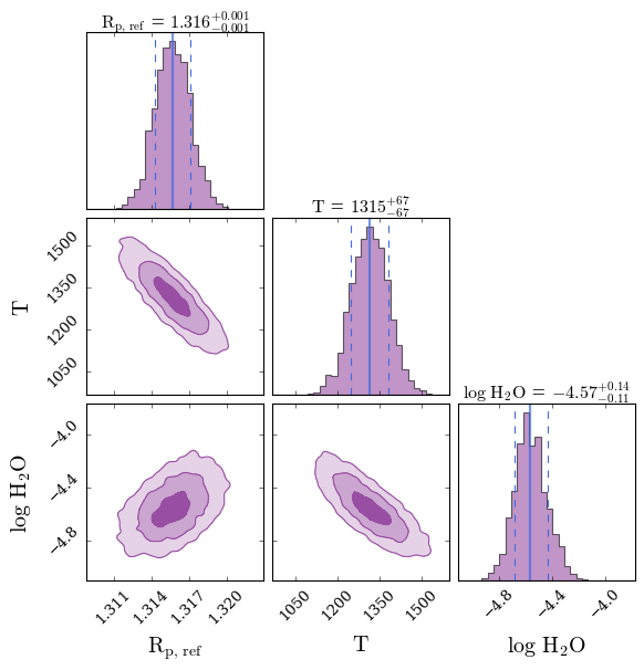
You first plot confidence intervals of the retrieved spectrum from this model compared to WASP-999b’s observed transmission spectrum. You also generate a corner plot showing the retrieved probability distributions of the model parameters.
[8]:
from POSEIDON.utility import read_retrieved_spectrum, plot_collection
from POSEIDON.visuals import plot_spectra_retrieved
from POSEIDON.corner import generate_cornerplot

#***** Plot retrieved transmission spectrum *****#

# Read retrieved spectrum confidence regions
wl, spec_low2, spec_low1, spec_median, \
spec_high1, spec_high2 = read_retrieved_spectrum(planet_name, model_name)

# Create composite spectra objects for plotting
spectra_median = plot_collection(spec_median, wl, collection = [])
spectra_low1 = plot_collection(spec_low1, wl, collection = [])
spectra_low2 = plot_collection(spec_low2, wl, collection = [])
spectra_high1 = plot_collection(spec_high1, wl, collection = [])
spectra_high2 = plot_collection(spec_high2, wl, collection = [])

# Produce figure
fig_spec = plot_spectra_retrieved(spectra_median, spectra_low2, spectra_low1,
                                  spectra_high1, spectra_high2, planet_name,
                                  data, R_to_bin = 100,
                                  data_labels = ['STIS G430', 'STIS G750', 'WFC3 G141'],
                                  data_colour_list = ['lime', 'cyan', 'black'])

#***** Make corner plot *****#

fig_corner = generate_cornerplot(planet, model)
Generating corner plot ...
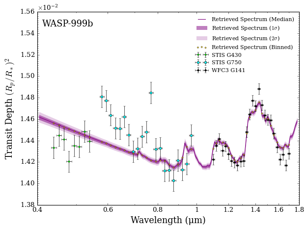
Not bad for a first simple model! The fit to the infrared WFC3 data looks reasonable, but there is considerable scatter in the visible wavelength data which isn’t captured by the model. You quantitatively assess the fit quality by opening the retrieval results file.
Tip:
Retrieval results are automatically created in the POSEIDON output directory, which will appear in the same directory as the Python file running POSEIDON.
The main retrieval results are found in
./POSEIDON_output/𝗽𝗹𝗮𝗻𝗲𝘁_𝗻𝗮𝗺𝗲/retrievals/results
There, you will find 2 files for each retrieval:
𝗺𝗼𝗱𝗲𝗹_𝗻𝗮𝗺𝗲_corner.pdf — the corner plot.
𝗺𝗼𝗱𝗲𝗹_𝗻𝗮𝗺𝗲_results.txt — a human-readable summary of the main retrieval results.
You can also find the posterior samples from the retrieval in
./POSEIDON_output/𝗽𝗹𝗮𝗻𝗲𝘁_𝗻𝗮𝗺𝗲/retrievals/samples
Inside the results file, you scroll down to the fit quality statistics.
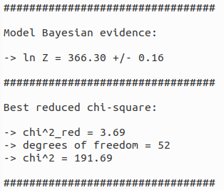
Well, that reduced \(\chi^2\) doesn’t look great… a value significantly greater than 1 likely indicates that your model is under fitting the observations.
Comparing Retrieval Fits
After a little reflection, you suspect the issue is that one or more chemical species with strong absorption cross sections at visible wavelengths is missing from the model. So you define a new model with \(\rm{Na}\), \(\rm{K}\), and \(\rm{TiO}\) added and run a second retrieval.
This 6-parameter retrieval should take about 20 minutes on a single core.
[9]:
#***** Define new model *****#

model_name_2 = 'Improved_retrieval'

bulk_species = ['H2', 'He']
param_species_2 = ['Na', 'K', 'TiO', 'H2O']  # Three new chemical species added

# Create the model object
model_2 = define_model(model_name_2, bulk_species, param_species_2,
                       PT_profile = 'isotherm', cloud_model = 'cloud-free')

# Check the free parameters defining this model
print("Free parameters: " + str(model_2['param_names']))

#***** Set priors for new retrieval *****#

# Initialise prior type dictionary
prior_types_2 = {}

# Specify whether priors are linear, Gaussian, etc.
prior_types_2['T'] = 'uniform'
prior_types_2['R_p_ref'] = 'uniform'
prior_types_2['log_X'] = 'uniform'    # 'log_X' sets the same prior for all mixing ratios

# Initialise prior range dictionary
prior_ranges_2 = {}

# Specify prior ranges for each free parameter
prior_ranges_2['T'] = [400, 1600]
prior_ranges_2['R_p_ref'] = [0.85*R_p, 1.15*R_p]
prior_ranges_2['log_X'] = [-12, -1]   # 'log_X' sets the same prior for all mixing ratios

# Create prior object for retrieval
priors_2 = set_priors(planet, star, model_2, data, prior_types_2, prior_ranges_2)

#***** Read opacity data *****#

# Pre-interpolate the opacities
opac_2 = read_opacities(model_2, wl, opacity_treatment, T_fine, log_P_fine)

#***** Run atmospheric retrieval *****#

run_retrieval(planet, star, model_2, opac_2, data, priors_2, wl, P, P_ref, R = R,
              spectrum_type = 'transmission', sampling_algorithm = 'MultiNest',
              N_live = 400, verbose = False)   # This last variable suppresses MultiNest terminal output
Free parameters: ['R_p_ref' 'T' 'log_Na' 'log_K' 'log_TiO' 'log_H2O']
Reading in cross sections in opacity sampling mode...
H2-H2 done
H2-He done
Na done
K done
TiO done
H2O done
Opacity pre-interpolation complete.
POSEIDON now running 'Improved_retrieval'
 *****************************************************
 MultiNest v3.10
 Copyright Farhan Feroz & Mike Hobson
 Release Jul 2015

 no. of live points =  400
 dimensionality =    6
 *****************************************************
POSEIDON retrieval finished in 0.28 hours ln(ev)=   430.53864549625445      +/-  0.19357264547510869
 Total Likelihood Evaluations:        30104
 Sampling finished. Exiting MultiNest

Now generating 1000 sampled spectra and P-T profiles from the posterior distribution...
This process will take approximately 0.52 minutes
All done! Output files can be found in ./POSEIDON_output/WASP-999b/retrievals/results/
Now that the new retrieval has finished, you compare the fit quality between the two models.
[10]:
#***** Plot retrieved transmission spectrum *****#

# Read retrieved spectrum confidence regions
wl, spec_low2, spec_low1, spec_median, \
spec_high1, spec_high2 = read_retrieved_spectrum(planet_name, model_name_2)

# Create composite spectra objects for plotting
spectra_median = plot_collection(spec_median, wl, collection = spectra_median)
spectra_low1 = plot_collection(spec_low1, wl, collection = spectra_low1)
spectra_low2 = plot_collection(spec_low2, wl, collection = spectra_low2)
spectra_high1 = plot_collection(spec_high1, wl, collection = spectra_high1)
spectra_high2 = plot_collection(spec_high2, wl, collection = spectra_high2)

# Produce figure
fig_spec = plot_spectra_retrieved(spectra_median, spectra_low2, spectra_low1,
                                  spectra_high1, spectra_high2, planet_name,
                                  data, R_to_bin = 100,
                                  spectra_labels = ['First Model', 'Add Alkalis'],
                                  data_labels = ['STIS G430', 'STIS G750', 'WFC3 G141'],
                                  data_colour_list = ['lime', 'cyan', 'black'])
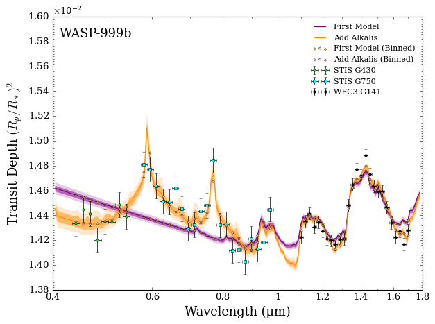
Now that looks like a much better fit! Checking the results file, you see that the Bayesian evidence for this new model is significantly higher and the reduced \(\chi^2\) is now much closer to 1.
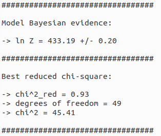
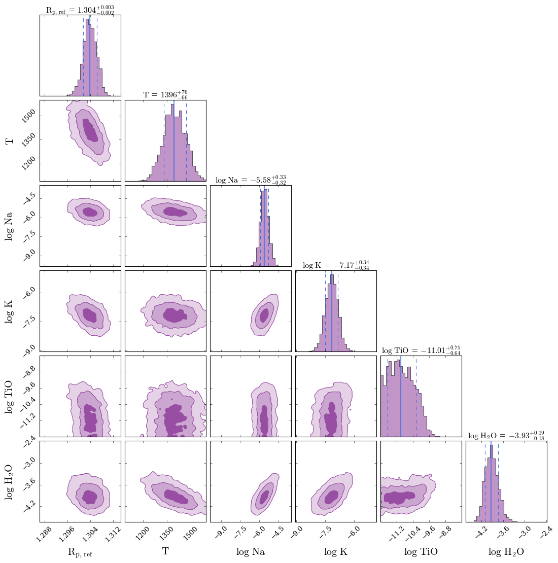
In fact, given that the reduced \(\chi^2 < 1\), this suggests a degree of over fitting. To see what is going on, you create a corner plot to visualise the retrieved parameters.
[11]:
fig_corner = generate_cornerplot(planet, model_2)
Generating corner plot ...
Bayesian Model Comparisons
What we have seen above are examples of Bayesian parameter estimation, represented by the corner plots (or more formally, the joint posterior probability distribution). Parameter estimation problems ask the question, “Given a model, what are the ranges of the model parameters that fit this dataset?”.
But we can also pose the question, “Given many models, which are better at explaining the data?”. This type of analysis is known as Bayesian model comparison.
Model Comparison Statistics
You already saw an example of a simple model comparison metric above (the reduced \(\chi^2\) of the best-fitting parameter combination), but we can go further. One of the by-products of a POSEIDON retrieval with MultiNest is the Bayesian evidence, \(\mathcal{Z}\), which is a global metric quantifying the quality of the model fit to the data (mathematically, the normalisation factor in the denominator of Bayes theorem). You actually saw the evidence values already in the screenshots from the POSEIDON ‘results.txt’ files.
While the Bayesian evidence of a single model isn’t informative, the ratio of the evidences of two nested models, the Bayes factor, \(\mathcal{B_{12}}\), tells us the probability (odds) ratio for the first model compared to the second model.
In the atmospheric retrieval literature, it is also common to see ‘frequentist equivalent’ detection significances quotes (expressed as a number of \(\sigma\)).
Chemical Detection Significances
Let’s now apply Bayesian model comparisons to answer the following question:
How confident are we that \(\rm{H}_2 \rm{O}\) and \(\rm{TiO}\) are in WASP-999b’s atmosphere?
To answer this, we first need to chose a reference model. Since our improved model above (with \(\rm{Na}\), \(\rm{K}\), \(\rm{TiO}\), and \(\rm{H}_2 \rm{O}\)) provides a good fit to the observations, we will adopt it as our reference model.
We will now run two more retrievals, both with the same setup as reference model but with (i) \(\rm{H}_2 \rm{O}\) removed and (ii) \(\rm{TiO}\) removed. These models are therefore nested models with respect to our reference model, since they have one less free parameter.
[15]:
#***** Define nested models *****#

model_name_3 = 'No_H2O'
model_name_4 = 'No_TiO'

param_species_3 = ['Na', 'K', 'TiO']  # No H2O
param_species_4 = ['Na', 'K', 'H2O']  # No TiO

# Create the model objects
model_3 = define_model(model_name_3, bulk_species, param_species_3,
                       PT_profile = 'isotherm', cloud_model = 'cloud-free')
model_4 = define_model(model_name_4, bulk_species, param_species_4,
                       PT_profile = 'isotherm', cloud_model = 'cloud-free')

# We can use the same priors as model 2 (since we used the same prior for all mixing ratios)

#***** Read opacity data *****#

# Pre-interpolate the opacities
opac_3 = read_opacities(model_3, wl, opacity_treatment, T_fine, log_P_fine)
opac_4 = read_opacities(model_4, wl, opacity_treatment, T_fine, log_P_fine)

#***** Run atmospheric retrievals *****#

# Retrieval with no H2O
run_retrieval(planet, star, model_3, opac_3, data, priors_2, wl, P, P_ref, R = R,   # Same priors as the reference model
              spectrum_type = 'transmission', sampling_algorithm = 'MultiNest',
              N_live = 400, verbose = False)

# Retrieval with no TiO
run_retrieval(planet, star, model_4, opac_4, data, priors_2, wl, P, P_ref, R = R,   # Same priors as the reference model
              spectrum_type = 'transmission', sampling_algorithm = 'MultiNest',
              N_live = 400, verbose = False)
Reading in cross sections in opacity sampling mode...
H2-H2 done
H2-He done
Na done
K done
TiO done
Opacity pre-interpolation complete.
Reading in cross sections in opacity sampling mode...
H2-H2 done
H2-He done
Na done
K done
H2O done
Opacity pre-interpolation complete.
POSEIDON now running 'No_H2O'
 *****************************************************
 MultiNest v3.10
 Copyright Farhan Feroz & Mike Hobson
 Release Jul 2015

 no. of live points =  400
 dimensionality =    5
 *****************************************************

 MultiNest Warning!
 Parameter            2  of mode            1  is converging towards the edge of the prior.

 MultiNest Warning!
 Parameter            2  of mode            1  is converging towards the edge of the prior.

 MultiNest Warning!
 Parameter            2  of mode            1  is converging towards the edge of the prior.

 MultiNest Warning!
 Parameter            2  of mode            1  is converging towards the edge of the prior.

 MultiNest Warning!
 Parameter            2  of mode            1  is converging towards the edge of the prior.

 MultiNest Warning!
 Parameter            2  of mode            1  is converging towards the edge of the prior.

 MultiNest Warning!
 Parameter            2  of mode            1  is converging towards the edge of the prior.

 MultiNest Warning!
 Parameter            2  of mode            1  is converging towards the edge of the prior.

 MultiNest Warning!
 Parameter            2  of mode            1  is converging towards the edge of the prior.

 MultiNest Warning!
 Parameter            2  of mode            1  is converging towards the edge of the prior.

 MultiNest Warning!
 Parameter            2  of mode            1  is converging towards the edge of the prior.

 MultiNest Warning!
 Parameter            2  of mode            1  is converging towards the edge of the prior.

 MultiNest Warning!
 Parameter            2  of mode            1  is converging towards the edge of the prior.

 MultiNest Warning!
 Parameter            2  of mode            1  is converging towards the edge of the prior.

 MultiNest Warning!
 Parameter            2  of mode            1  is converging towards the edge of the prior.

 MultiNest Warning!
 Parameter            2  of mode            1  is converging towards the edge of the prior.

 MultiNest Warning!
 Parameter            2  of mode            1  is converging towards the edge of the prior.

 MultiNest Warning!
 Parameter            2  of mode            1  is converging towards the edge of the prior.

 MultiNest Warning!
 Parameter            2  of mode            1  is converging towards the edge of the prior.

 MultiNest Warning!
 Parameter            2  of mode            1  is converging towards the edge of the prior.

 MultiNest Warning!
 Parameter            2  of mode            1  is converging towards the edge of the prior.

 MultiNest Warning!
 Parameter            2  of mode            1  is converging towards the edge of the prior.

 MultiNest Warning!
 Parameter            2  of mode            1  is converging towards the edge of the prior.

 MultiNest Warning!
 Parameter            2  of mode            1  is converging towards the edge of the prior.

 MultiNest Warning!
 Parameter            2  of mode            1  is converging towards the edge of the prior.

 MultiNest Warning!
 Parameter            2  of mode            1  is converging towards the edge of the prior.

 MultiNest Warning!
 Parameter            2  of mode            1  is converging towards the edge of the prior.

 MultiNest Warning!
 Parameter            2  of mode            1  is converging towards the edge of the prior.

 MultiNest Warning!
 Parameter            2  of mode            1  is converging towards the edge of the prior.

 MultiNest Warning!
 Parameter            2  of mode            1  is converging towards the edge of the prior.
POSEIDON retrieval finished in 0.077 hours ln(ev)=   163.17107197349620      +/-  0.19198690162212451
 Total Likelihood Evaluations:        15370
 Sampling finished. Exiting MultiNest

Now generating 1000 sampled spectra and P-T profiles from the posterior distribution...
This process will take approximately 0.34 minutes
All done! Output files can be found in ./POSEIDON_output/WASP-999b/retrievals/results/
POSEIDON now running 'No_TiO'
 *****************************************************
 MultiNest v3.10
 Copyright Farhan Feroz & Mike Hobson
 Release Jul 2015

 no. of live points =  400
 dimensionality =    5
 *****************************************************
POSEIDON retrieval finished in 0.098 hours ln(ev)=   434.15573682621977      +/-  0.18891786537003397
 Total Likelihood Evaluations:        19226
 Sampling finished. Exiting MultiNest

Now generating 1000 sampled spectra and P-T profiles from the posterior distribution...
This process will take approximately 0.32 minutes
All done! Output files can be found in ./POSEIDON_output/WASP-999b/retrievals/results/
(By the way, when MultiNest prints out convergence warnings like those above it is a clue telling you the fit is so bad that another free parameter is being forced to the edge of the prior — in this case, it is because \(\rm{H}_2 \rm{O}\) is the only infrared opacity source so it really needs to be included in the model!)
POSEIDON includes a convenient function we can use to carry out Bayesian model comparisons.
[16]:
from POSEIDON.retrieval import Bayesian_model_comparison

# Rename the models just for convenience
model_ref = model_2
model_no_H2O = model_3
model_no_TiO = model_4

# H2O model comparison
Bayesian_model_comparison(planet_name, model_ref, model_no_H2O)
Bayesian evidences:

Model Improved_retrieval: ln Z = 433.21 +/- 0.19
Model No_H2O: ln Z = 163.17 +/- 0.19

Bayes factor:

B = 1.89e+117
ln B = 270.04

'Equivalent' detection significance:

23.4 σ
[17]:
# TiO model comparison
Bayesian_model_comparison(planet_name, model_ref, model_no_TiO)
Bayesian evidences:

Model Improved_retrieval: ln Z = 433.21 +/- 0.19
Model No_TiO: ln Z = 434.16 +/- 0.19

Bayes factor:

B = 3.89e-01
ln B = -0.94

No detection of the reference model, model No_TiO is preferred.
So the Bayesian model comparisons tell us we have a strong detection of \(\rm{H}_2 \rm{O}\) but no evidence for \(\rm{TiO}\). Indeed, the Bayesian evidence actually improves when we remove \(\rm{TiO}\).
The tendency of the Bayesian evidence to lower when including redundant parameters, sometimes called the ‘Occam penalty’, is one of the powerful features of the Bayesian evidence in finding the optimal model to explain a given dataset.
To gain intuition for why the model comparison so strongly favours \(\rm{H}_2 \rm{O}\), let’s plot the retrieved spectra.
[18]:
# Read retrieved spectrum confidence regions
wl, spec_low2, spec_low1, spec_median, \
spec_high1, spec_high2 = read_retrieved_spectrum(planet_name, model_ref['model_name'])

# Create composite spectra objects for plotting
spectra_median = plot_collection(spec_median, wl, collection = [])
spectra_low1 = plot_collection(spec_low1, wl, collection = [])
spectra_low2 = plot_collection(spec_low2, wl, collection = [])
spectra_high1 = plot_collection(spec_high1, wl, collection = [])
spectra_high2 = plot_collection(spec_high2, wl, collection = [])

# Read retrieved spectrum confidence regions
wl, spec_low2, spec_low1, spec_median, \
spec_high1, spec_high2 = read_retrieved_spectrum(planet_name, model_no_H2O['model_name'])

# Create composite spectra objects for plotting
spectra_median = plot_collection(spec_median, wl, collection = spectra_median)
spectra_low1 = plot_collection(spec_low1, wl, collection = spectra_low1)
spectra_low2 = plot_collection(spec_low2, wl, collection = spectra_low2)
spectra_high1 = plot_collection(spec_high1, wl, collection = spectra_high1)
spectra_high2 = plot_collection(spec_high2, wl, collection = spectra_high2)

# Produce figure
fig_spec = plot_spectra_retrieved(spectra_median, spectra_low2, spectra_low1,
                                  spectra_high1, spectra_high2, planet_name,
                                  data, R_to_bin = 100,
                                  spectra_labels = ['Reference model', 'No H$_2$O'],
                                  data_labels = ['STIS G430', 'STIS G750', 'WFC3 G141'],
                                  data_colour_list = ['lime', 'cyan', 'black'],
                                  plt_label = 'Effect of Removing H$_2$O')
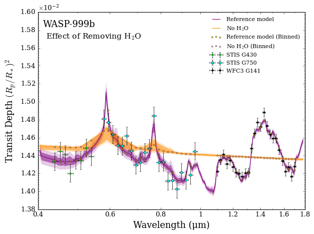
As you can see, even when the retrieval tries its best to minimise the residuals, without \(\rm{H}_2 \rm{O}\) there is simply no way to explain the data. This is the kind of scenario that results in a 23 σ detection.
What about \(\rm{TiO}\)?
[19]:
# Read retrieved spectrum confidence regions
wl, spec_low2, spec_low1, spec_median, \
spec_high1, spec_high2 = read_retrieved_spectrum(planet_name, model_ref['model_name'])

# Create composite spectra objects for plotting
spectra_median = plot_collection(spec_median, wl, collection = [])
spectra_low1 = plot_collection(spec_low1, wl, collection = [])
spectra_low2 = plot_collection(spec_low2, wl, collection = [])
spectra_high1 = plot_collection(spec_high1, wl, collection = [])
spectra_high2 = plot_collection(spec_high2, wl, collection = [])

# Read retrieved spectrum confidence regions
wl, spec_low2, spec_low1, spec_median, \
spec_high1, spec_high2 = read_retrieved_spectrum(planet_name, model_no_TiO['model_name'])

# Create composite spectra objects for plotting
spectra_median = plot_collection(spec_median, wl, collection = spectra_median)
spectra_low1 = plot_collection(spec_low1, wl, collection = spectra_low1)
spectra_low2 = plot_collection(spec_low2, wl, collection = spectra_low2)
spectra_high1 = plot_collection(spec_high1, wl, collection = spectra_high1)
spectra_high2 = plot_collection(spec_high2, wl, collection = spectra_high2)

# Produce figure
fig_spec = plot_spectra_retrieved(spectra_median, spectra_low2, spectra_low1,
                                  spectra_high1, spectra_high2, planet_name,
                                  data, R_to_bin = 100,
                                  spectra_labels = ['Reference model', 'No TiO'],
                                  data_labels = ['STIS G430', 'STIS G750', 'WFC3 G141'],
                                  data_colour_list = ['lime', 'cyan', 'black'],
                                  plt_label = 'Effect of Removing TiO')
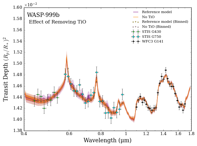
The retrieved spectrum looks almost the same, but with the possibility of \(\rm{TiO}\) bands no longer showing in the visible wavelengths. Since the overall quality of the fits are essentially the same, the Bayesian evidence favours the simpler model without \(\rm{TiO}\).