Note

Download full notebook here

Ground-Based High-Resolution Emission Spectroscopy (Cross Correlation)

This tutorial covers how to run cross-correlation analysis with high resolution data using POSEIDON. We will reproduce the result from Brogi and Line 2019, validating our framework with the \(\rm{H}_2\rm{O}\) and \(\rm{CO}_2\) detection on WASP-77Ab.

Following from the previous tutorial, we will now work with emission spectroscopy. Thus, rather than having the planet crossing in front of the stellar disk, it will be observed approximately half-orbit later, when the dayside of the planet is in full view.

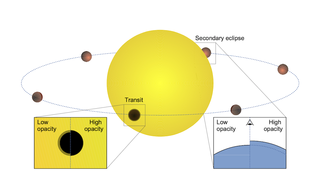
NOTE: At low spectral resolution (e.g. HST/WFC3, JWST) and in photometry (i.e. Spitzer IRAC), you are used to think to the planet’s emission measured as the drop in flux during secondary eclipse. In HR spectroscopy, we can’t accurately measure secondary eclipses because of the low SNR. We instead observe before or after secondary eclipse, i.e. when both the stellar and the planet spectrum are present.

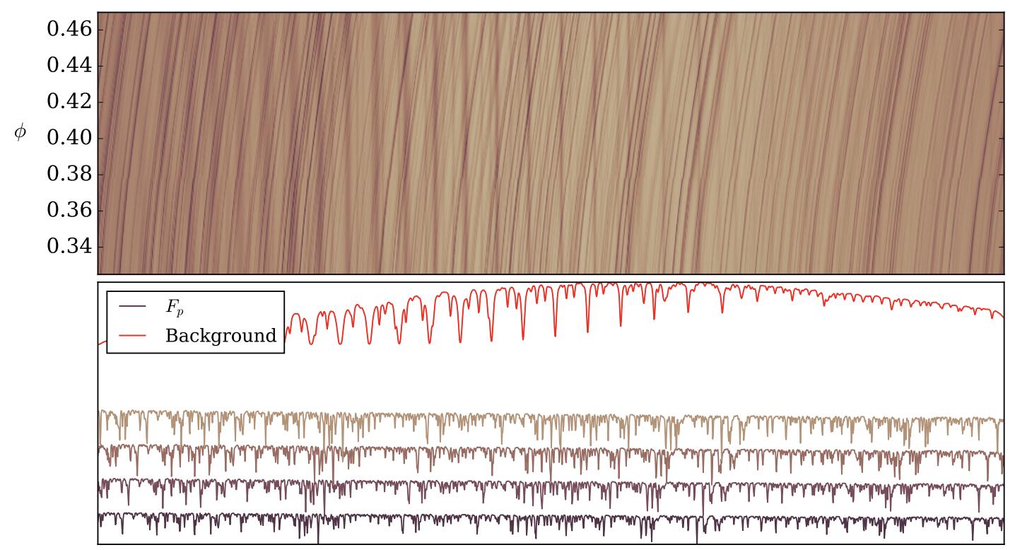
RECALL: What allows us to separate the two is the changing Doppler shift of the spectrum. This is explained by the figure below, where the telluric and stellar lines (stationary in wavelengths) are in the background and the planet’s lines (Doppler-shifting) are in the foreground. The observed data is essentially a noise sum of the two, and our job to the extract the Doppler-shifting planet signals!

Since we do not need the secondary eclipse anymore, HR emission spectroscopy can also be done on non-transiting planets.

Loading WASP-77Ab Emission Data

We start from a wavelength-aligned raw flux from the observation of our planet (WASP-77Ab). The data used in this tutorial should be under your data directory +”/IGRINS/data_raw.hdf5”. We support analysis with combined multiple observations. To see how this could be done, see the transmission high-resolution retireval tutorial.

Your data should include

1. raw flux from the observation, This should be a 3D array: NOrders x NExposures x NPixels.

2. wavelength grid of your observations. This should be a 2D array: NOrders x Npixels.

3. orbital phase of each exposure. This should be a 1D array: NExposures.

Suppose this is the first time you use POSEIDON on this dataset. We will read the dataset in its raw form, processes it, and save it into POSEIDON compatibale format (.hdf5).

Reminder: POSEIDON calculates spectra in vacuum wavelengths. If your data come in air wavelengths, you could use POSEIDON.high_res.airtovac for wavelength conversion.

from POSEIDON.high_res import fit_uncertainties, read_hdf5

planet_name = "WASP-77Ab"

data_dir = '../../../POSEIDON/reference_data/observations/' + planet_name # Special directory for this tutorial

name = "IGRINS"

data_raw = read_hdf5(data_dir + "/" + name + "/data_raw.hdf5")
flux = data_raw["flux"]
wl_grid = data_raw["wl_grid"]
phi = data_raw["phi"]
V_bary = data_raw["V_bary"]

print(data_raw.keys())

dict_keys(['V_bary', 'flux', 'phi', 'wl_grid'])

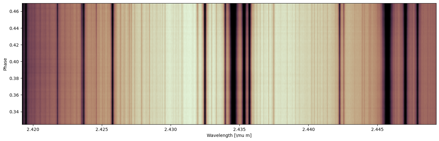
Visualizing data

We start from a wavelength-aligned, preprocessed high resolution raw flux for our planet (WASP-77Ab). The data used in this tutorial should be under your directory +”/IGRINS/data_processed.hdf5”. We support analysis with combined multiple observations. To see how this could be done, see the transmission high-resolution retireval tutorial.

import matplotlib.pyplot as plt
import numpy as np
import cmasher as cmr

cmap = cmr.sepia
plt.figure(figsize=(17, 5))
plt.imshow(flux[0], aspect="auto", origin="lower", cmap=cmap,
    extent=[wl_grid[0][0], wl_grid[0][-1], phi[0], phi[-1]])
plt.ticklabel_format(useOffset=False)
plt.xlabel(r"Wavelength [\mu m]")
plt.ylabel("Phase")
plt.show()

Preparing Data From Raw Flux

The above data used for the tutorial is already processed with “prepare_high_res_data”. When you perform your analysis on a new dataset, you need to call this function that will perform PCA or SYSREM to filter the data and save at given directory. To use PCA instead of SYSREM, change ‘sysrem’ into ‘pca’. No more changes are needed for other part of the code. Notice that PCA filtering does not acccount for time-wavelength dependent uncertainties and therefore we do not need to fit for the uncertainties.

from POSEIDON.high_res import prepare_high_res_data
uncertainties = fit_uncertainties(flux, initial_guess=[0.01, np.mean(flux)])
prepare_high_res_data(data_dir, name, "emission", "sysrem", flux, wl_grid,
                      phi, uncertainties, transit_weight=None, V_bary=V_bary)  # This data set is not barycentric corrected, therefore we provide the barycentric velocity

Configuring the Forward Model

Below, we are setting up POSEIDON’s forward model. This includes specifying the the properties of the star-planet system, which chemical species we want to include, the resolution at which we calculate the model, and the temperature-pressure profile of our model atmosphere.

Here we set the spectral resolution to be R=250,000. This is a tradeoff between speed (also RAM) and accuracy. Because our high-dispersion data usually has R ≥ 25,000, empirically we want our model to be 10 times more refined than the data such that when binned down to data resolution, it retains high accuracy.

For more advanced usage of POSEIDON’s emission forward model, see the “Thermal Scattering” tutorial.

Then, let’s provide the wavelength grid and properties of the host star and your planet. The wavelength range should match the range of your data. This observation spans 1.3 microns to 2.6 microns.

from POSEIDON.core import create_planet, create_star , make_atmosphere, read_opacities, \
                          compute_spectrum, define_model, wl_grid_constant_R

from POSEIDON.constants import R_Sun, R_J, M_J

# ***** Define stellar properties *****#

R_s = 0.91 * R_Sun  # Stellar radius (m)
T_s = 5605.0        # Stellar effective temperature (K)
Met_s = -0.04       # Stellar metallicity [log10(Fe/H_star / Fe/H_solar)]
log_g_s = 4.48      # Stellar log surface gravity (log10(cm/s^2) by convention)

# ***** Define planet properties *****#

planet_name = "WASP-77Ab"  # Planet name used for plots, output files etc.

R_p = 1.21 * R_J  # Planetary radius (m)
M_p = 1.76 * M_J  # Mass of planet (kg)

# Create the planet object
planet = create_planet(planet_name, R_p, mass=M_p)

# If distance not specified, use fiducial value
if planet["system_distance"] is None:
    planet["system_distance"] = 1  # This value only used for flux ratios, so it cancels
d = planet["system_distance"]

Existing literature have shown detection of \(\rm{H}_2\rm{O}\) and \(\rm{C}\rm{O}_2\) in the atmosphere of WASP-77Ab.

So for a first attempt, we consider a model with \(\rm{H}_2\rm{O}\) and \(\rm{C}\rm{O}_2\), an isothermal temperature profile, and no clouds.

For additional parameters used in high resolution retrieval, we include: \(log_\alpha\) (the scaling parameter), \(K_p\) (the Keplerian orbital velocity), \(V_{sys}\) (the systematic velocity), and \(W_{conv}\) (width of the gaussian convolution kernel used for line broadening). Additional parameters available are \(\Delta \phi\) (offseting the ephemeris) and b (the scaling parameter for noise).

model_name = "Cross Correlation"  # Model name used for plots, output files etc.
bulk_species = ["H2", "He"]  # H2 + He comprises the bulk atmosphere

param_species = ["H2O", "CO"]

model = define_model(model_name, bulk_species, param_species,
                    PT_profile="Madhu", reference_parameter="R_p_ref")

# ***** Wavelength grid *****#

wl_min = 1.3   # Minimum wavelength (um)
wl_max = 2.6   # Maximum wavelength (um)
R = 250000      # Spectral resolution of the model wavelength grid
                # Note: for high-res data, the resolution of the grid is recommended
                # to be 10x higher than the data. Since we are dealing with high-res data
                # with R~80,000, R=250,000 is a good tradeoff between RAM, computational speed and accuracy

wl = wl_grid_constant_R(wl_min, wl_max, R)

# ***** Read opacity data *****#
opacity_treatment = "opacity_sampling"

# Define fine temperature grid (K)
T_fine_min = 400   # 400 K lower limit suffices for a typical hot Jupiter
T_fine_max = 4000  # 2000 K upper limit suffices for a typical hot Jupiter
T_fine_step = 50   # 20 K steps are a good tradeoff between accuracy and RAM

T_fine = np.arange(T_fine_min, (T_fine_max + T_fine_step), T_fine_step)

# Define fine pressure grid (log10(P/bar))
log_P_fine_min = -5.0  # 1 ubar is the lowest pressure in the opacity database
log_P_fine_max = 2     # 100 bar is the highest pressure in the opacity database
log_P_fine_step = 0.2  # 0.2 dex steps are a good tradeoff between accuracy and RAM

log_P_fine = np.arange(log_P_fine_min, (log_P_fine_max + log_P_fine_step), log_P_fine_step)

opac = read_opacities(model, wl, opacity_treatment, T_fine, log_P_fine)

Reading in cross sections in opacity sampling mode...
H2-H2 done
H2-He done
H2O done
CO done
Opacity pre-interpolation complete.

Generating an emission spectrum and cross-correlating with data

To do so, you need to specify the atmosphere setting and provide values for your model parameters. We can the cross-correlate the spectrum we created with the processed data we obtained from running “prepare_high_res_data”. We can plot the cross-correlating function as a function of \(K_p\) and \(V_{sys}\) and see the peak at the expected location. If you want to run retrieval only, you can remove the cells from this section.

# ***** Specify fixed atmospheric settings for retrieval *****#
# Specify the pressure grid of the atmosphere
P_min = 1.0e-5  # 0.1 ubar
P_max = 100     # 100 bar
N_layers = 100  # 100 layers

# We'll space the layers uniformly in log-pressure
P = np.logspace(np.log10(P_max), np.log10(P_min), N_layers)

# Specify the reference pressure and radius
P_ref = 1e-2   # Reference pressure (bar)
R_p_ref = R_p  # Radius at reference pressure

log_species = [-4, -4]

# Provide a specific set of model parameters for the atmosphere
PT_params = np.array(
    [0.2, 0.1, 0.17, -1.39, 1, 1500]
)  # a1, a2, log_P1, log_P2, log_P3, T_top
log_X_params = np.array([log_species])

atmosphere = make_atmosphere(planet, model, P, P_ref, R_p_ref, PT_params,
                             log_X_params, P_param_set=1e-5)

# Create the stellar object
star = create_star(R_s, T_s, log_g_s, Met_s, wl=wl, stellar_grid="phoenix")

# Generate planet surface flux
spectrum = compute_spectrum(planet, star, model, atmosphere, opac, wl,
                            spectrum_type="direct_emission")

Cross-Correlation

Cross correlation has been used in various flavours since the first application in Snellen et al. 2010. In this example, we use the following definition:

\[CCF(v,t) = \sum_i^N \frac{ f_i(t) m_i(v)}{\sigma_i^2}\]

Here, \(m_i\) is the template shifted to a radial velocity \(v\). \(f_i\) is the residual observed at time \(t\). \(m_i\) is now defined on the same grid as \(f_i\) through interpolation. \(C\) then is a 2-dimensional matrix, as function of time along the transit and the radial velocity shift of the template. At the correct combination of time and velocity, the signal of the planet should appear.

Let’s cross-correlate our template model with the data!

from POSEIDON.high_res import cross_correlate, read_high_res_data

name = "IGRINS"

data = read_high_res_data(data_dir, names=[name])
data[name]["uncertainties"] = np.ones_like(flux) # Not weighted by uncertainties to reproduce Brogi & Line 2019

Kp_range = np.arange(0, 301, 1)
Vsys_range = np.arange(-100, 101, 1)
RV_range = np.arange(-100, 401, 1)   # Set RV range to (min(Kp)+min(Vsys), max(Kp)+max(Vsys))

CCF_Kp_Vsys_all = []
CCF_phase_RV_all = []

# Loop through all the data sets and cross correlate them with the model spectrum
for key in data.keys():
    CCF_Kp_Vsys, CCF_phase_RV = cross_correlate(Kp_range, Vsys_range, RV_range, wl, spectrum, data[key])
    CCF_Kp_Vsys_all.append(CCF_Kp_Vsys)
    CCF_phase_RV_all.append(CCF_phase_RV)

CCF_phase_RV_all = np.array(CCF_phase_RV_all)
CCF_Kp_Vsys_all = np.array(CCF_Kp_Vsys_all)

Cross correlation took 33.22029519081116 seconds

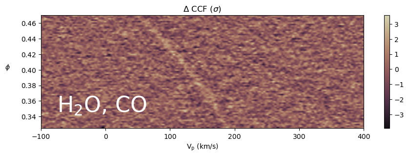
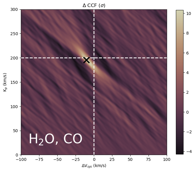
Below we plot CCF as a function of \(V_p\) and phase \(\phi\). Ideally, we could see a trail with slope \(\approx K_p\) and \(V_p(\phi=0) \approx V_{sys}\) in the CCF space. Phase-folding this plot given a \(K_p\) gives rise to one single row in the \(K_p-V_{sys}\) plot above.

from POSEIDON.high_res import plot_CCF_Kp_Vsys, plot_CCF_phase_RV

# Plotting the CCF_Kp map after summing up all the datasets
plot_CCF_Kp_Vsys(Kp_range, Vsys_range, CCF_Kp_Vsys=np.sum(CCF_Kp_Vsys_all[:], axis=0),
                 label=r"$\rm{H_2}$O, CO", Kp_expected=200, Vsys_expected=0, RM_mask_size=20,
                 plot_slice=True, save_file_path=None, cmap=cmr.get_sub_cmap("cmr.sepia", 0.1, 0.9))

plot_CCF_phase_RV(phi, RV_range, np.mean(CCF_phase_RV_all, axis=0), label=r"$\rm{H_2}$O, CO",
                  save_filepath=None, cmap=cmr.get_sub_cmap("cmr.sepia", 0.1, 0.9))